Download

1 / 52
550 likes | 573 Views
Texture Mapping. CMSC435 UMBC. *With lots of borrowing from the usual victims…. Motivation. Flat and Boring. “ Textured ”. Texture Mapping. Definition: mapping a function onto a surface; function can be: 1, 2, or 3D sampled (image) or mathematical function. Texture Mapping.

E N D
Texture Mapping CMSC435 UMBC *With lots of borrowing from the usual victims…
Motivation Flat and Boring “Textured”
Texture Mapping • Definition: mapping a function onto a surface; function can be: • 1, 2, or 3D • sampled (image) or mathematical function
Texture Mapping “Texture” Boring Geometry Texture An image that’s mapped onto something Texel Texture pixel (Also, an island in Denmark…)
Texture Mapping Interesting Geometry
Texture Mapping Mapping Function 2D Texture Coordinate 3D Coordinate Texture Image
Texture Coordinates u • Normalized 2D space • 0-1 on each axis • Letters vary: • U,V are most common • GL/RMan specs like s,t • Typically periodic D3D v Texture Coordinates as RGB OGL t s
0,0 0,0 0,0 0,0 0,1 0,4 0,8 0,2 1,0 4,0 8,0 2,0 Texture Tiling Scale UV Coordinates Alter texture frequency
Planar Mapping • For xy aligned plane • Reverse projection 9
Cylindrical Mapping • For cylinder with point • Texture coordinates 11
Spherical Mapping • For sphere with point • Texture coordinates 13
Mapping onto Parametric Patches Use scaled surface u,v parameters for texture u,v 15
Mapping onto Polygons Explicit per-vertex coordinates… Wikipedia
Properties of good UV layout: Minimizes stretch Maximize packing efficiency Easy for artist to paint into Unlike that one… Automatic is possible, but manual often preferred Texture Atlas Zhou et al.
Texture Atlas Not always a 1:1 mapping
Discontinuity at UV chart boundaries Solutions: Fix them: Copy/Blend texels across boundary Hide them Armpits, ankles, backs of heads, under clothing Texture Seams Peter Kojesta (Gamasutra)
Environment Mapping Surround scene with maps simulating surrounding detail 21
Distant Reflection Look up reflection direction in reflection or environment map 22
Pick a face based on largest normal component Project onto the face Divide through Use resulting coordinates for 2D lookup Cubic Environment Maps
Photograph of shiny sphere Lookup based on x/y coordinates of normal Spherical Environment Maps DirectX Documentation
Texture All the Things • Texture/Albedo map (Catmull 74) • Reflection Map (Blinn and Newell 76) • Bump/Normal Map (Blinn78 / Cohen 98) • Gloss Map (Blinn 78) • Transparency Map (Gardner 85) • Diffuse Reflectance (Miller and Hoffman 84) • Shadows, displacements, etc (Cook 84) • Tangent map (Kajiya 85)
Point Sampling Map UV coordinate onto texel grid, grab corresponding texel i = floor(u*width) j = floor(v*height) Just like in 1995 Texture Sampling
Point Sampling Point sampling under magnification
Bilinear Filtering Interpolate texels in 2x2 neighborhood Top-left texel: floor(u*(width-1)), floor(v*(height-1)) Weight by fractional coordinates Filtered Sampling
Point Sampling Point sampling under magnification
Linear Sampling Linear sampling under magnification
Array of 2D slices 3D Coordinates (u,v,w) Bilinear tap in each slice using u,v Blend using w 3D Textures
Minification Aliasing! Pixels:Texels < 1: Minification Pixels:Texels ~= 1 Pixels:Texels > 1: Magnification
Anti-aliasing problem Minification Filtering Projected pixel footprint Texel grid Large jumps between pixels. Texture is undersampled…
One solution: Average lots of samples Minification Filtering Problems: - Expensive - Guessing the right sampling rate - Performance death spiral for heavy minification
Prefiltering: Precalculate chain of filtered images Each level is ½ previous resolution Mip-Mapping From Latin: "multum in parvo" (much in little)
Memory overhead is 33% Level i+1 is ½ resolution of i: W/2*H/2=WH/4 So… Mip-Mapping Geometric series
Derive footprint using UV derivatives in screenspace Mip-Mapping du/dy, dv/dy du/dx, dv/dx
Approximate footprint with a square W = Width of square in texels Find mip level matching footprint size Mip-Mapping w
Mip-Mapping Width of square in texels Finest level that won’t alias Base texels per ith level texel Magnification “Just Right” Aliasing 0 Level of detail …
Mip-Mapping Level i Blend bilinear taps at two nearest levels (8 texels accessed) Sometimes incorrectly called “Trilinear” Increasing footprint size Level i+1
Getting Derivatives • Rasterizer: 2x2 Quads + Differencing Missing pixels are extrapolated… Each 2x2 quad is self-contained This is a collosal pain in the collective necks of hardware architects
Raytracer Intersect “differential” rays with tangent plane Track derivatives during secondary bounces Getting Derivatives
Mip-Mapping • Advantages: • Cheap approximation to super-sampling • Ensures 1:1 pixel/texel ratio • May actually be FASTER than bilinear • Avoids cache thrashing
Mip-Mapping • Disadvantages: • Needs derivatives • Complicates renderer • 33% Memory overhead • Needs some preprocessing
Mipmapping is isotropic Same in all directions At oblique angles, footprint is NOT isotropic Result: Too much blur Anisotropic Filtering
“Ideal” solution: Elliptical Weighted Average (EWA) Anisotropic gaussian kernel “Gold Standard” Anisotropic Filtering
Actual Solution: Approximate ellipse with rectangle Box kernel Minor axis picks level Multiple filter taps along major axis Anisotropic Filtering 4x Anisotropic