Download
1 / 52
560 likes | 732 Views
Knowledge Technologies. Background in geospatial data modeling. Dept. of Informatics and Telecommunications National and Kapodistrian University of Athens. Outline. Basic GIS concepts and terminology Geographic space modeling paradigms Geospatial data standards. 2.

E N D
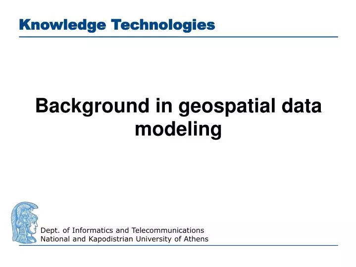
Knowledge Technologies Background in geospatial data modeling Dept. of Informatics and Telecommunications National and Kapodistrian University of Athens
Outline • Basic GIS concepts and terminology • Geographic space modeling paradigms • Geospatial data standards 2
Basic GIS Concepts and Terminology • Theme: the information corresponding to a particular domain that we want to model. A theme is a set of geographic features. • Example: the countries of Europe 3
Basic GIS Concepts (cont’d) • Geographic feature or geographic object: a domain entity that can have various attributes that describe spatialand non-spatial characteristics. • Example: the country Greece with attributes • Population • Flag • Capital • Geographical area • Coastline • Bordering countries 4
Basic GIS Concepts (cont’d) • Geographic features can be atomic or complex. • Example: According to the Kallikratis administrative reform of 2010, Greece consists of: • 13 regions (e.g., Crete) • Each region consists of perfectures (e.g., Heraklion) • Each perfecture consists of municipalities (e.g., DimosChersonisou) 5
Basic GIS Concepts (cont’d) • The spatial characteristics of a feature can involve: • Geometric information (location in the underlying geographic space, shape etc.) • Topological information (containment, adjacency etc.). Municipalities of the perfecture of Heraklion: 1. Dimos Irakliou2. Dimos Archanon-Asterousion3. Dimos Viannou4. Dimos Gortynas5. Dimos Maleviziou6. Dimos Minoa Pediadas7. Dimos Festou8. Dimos Chersonisou 6
Geometric Information • Geometric information can be captured by using geometric primitives (points, lines, polygons, etc.) to approximate the spatial attributes of the real world feature that we want to model. • Geometries are associated with a coordinate reference system which describes the coordinate space in which the geometry is defined. 7
Topological Information • Topological information is inherently qualitative and it is expressed in terms of topological relations (e.g., containment, adjacency, overlap etc.). • Topological information can be derived from geometric information or it might be captured by asserting explicitly the topological relations between features. 8
Topological Relations • The study of topological relations has produced a lot of interesting results by researchers in: • GIS • Spatial databases • Artificial Intelligence (qualitative reasoning and knowledge representation) 9
The 4-intersection model • The 4-intersection model has been defined by Egenhofer and Franzosa in 1991 based on previous work by Egenhofer and colleagues. • It is based on point-set topology. • Spatial regions are defined to be non-empty, proper subsets of a topological space. In addition, they must be closed and have connected interiors. • Topological relations are the ones that are invariant under topological homeomorphisms. 10
4IM and 9IM • The 4-intersection model can captures topological relations between two spatial regions a and b by considering whetherthe intersection of their boundaries and interiors is empty or non-empty. • The 9-intersection model is an extension of the 4-intersection model (Egenhofer and Herring, 1991). • 9IM captures topological relations between two spatial regions a and b by considering whether the intersection of their boundaries, interiors and exteriors is empty or non-empty. 11
DE-9IM • The dimensionally extended 9-intersection model has been defined by Clementini and Felice in 1994. • It is also based on the point-set topology of R2 and deals with “simple”, closed geometries (areas, lines, points). • Like its predecessors (4IM, 9IM), it can also be extended to more complex geometries (areas with holes, geometries with multiple components). 12
DE-9IM • It captures topological relationships between two geometries a and b in R2 by considering the dimensions of the intersections of the boundaries, interiors and exteriors of the two geometries: • The dimension can be 2, 1, 0 and -1 (dimension of the empty set). 13
DE-9IM • Five jointly exclusive and pairwise disjoint (JEPD) relationships between two different geometries can be distinguished (disjoint, touches, crosses, within, overlaps). • The modelcan also be defined using an appropriate calculus of geometries that uses these 5 binary relations and boundary operators. • See the paper: E. Clementini and P. Felice. A Comparison of Methods for Representing Topological Relationships. Information Sciences 80 (1994), pp. 1-34. 14
Example: A disjoint C A C • Notation: • T = { 0, 1, 2 } • F = -1 • * = don’t care = { -1, 0, 1, 2 } 15
Example: A within C C A • Notation equivalent to 3x3 matrix: • String of 9 characters representing the above matrix in row major order. • In this case: T*F**F*** 16
The Region Connection Calculus (RCC) • The primitives of the calculus are spatial regions. These are non-empty, regular subsets of a topological space. • The calculus is based on a single binary predicate C that formalizes the “connectedness” relation. • C(a,b)is true when the closure of a is connected to the closure of b i.e., they have at least one point in common. • It is axiomatized using first order logic. • See the original paper by Randell, Cui and Cohn (KR 1991). 18
RCC-8 • This is a set of eight JEPD binary relations that can be defined in terms of predicate C. 19
RCC-5 • The RCC-5 subset has also been studied. The granularity here is coarser. The boundary of a region is not taken into consideration: • No distinction among DC and EC, called just DR. • No distinction among TPP and NTPP, called just PP. • RCC-8 and RCC-5 relations can also be defined using point-set topology, and there are very close connections to the models of Egenhofer and others. 20
More Qualitative Spatial Relations • Orientation/Cardinal directions (left of, right of, north of, south of, northeast of etc.) • Distance (close to, far from etc.). This information can also be quantitative. 21
Coordinate Systems • Coordinate: one of n scalar values that determines the position of a point in an n-dimensional space. • Coordinate system: a set of mathematical rules for specifying how coordinates are to be assigned to points. • Example: the Cartesian coordinate system 22
Coordinate Reference Systems • Coordinate reference system: a coordinate system that is related to an object (e.g., the Earth, a planar projection of the Earth, a three dimensional mathematical space such as R3) through a datum which species its origin, scale, and orientation. • The term spatial reference system is also used. 23
Geographic Coordinate Reference Systems • These are 3-dimensional coordinate systems that utilize latitude (φ), longitude (λ) , and optionally geodetic height (i.e., elevation), to capture geographic locations on Earth. 24
The World Geodetic System • The World Geodetic System (WGS) is the most well-known geographic coordinate reference system and its latest revision is WGS84. • Applications: cartography, geodesy, navigation (GPS), etc. 25
Projected Coordinate Reference Systems • Projected coordinate reference system: they transform the 3-dimensional approximation of the Earth into a 2-dimensional surface (distortions!) • Example: the Universal Transverse Mercator (UTM) system 26
Coordinate Reference Systems (cont’d) • There are well-known ways to translate between co-ordinate reference systems. • Various authorities maintain lists of coordinate reference systems. See for example: • OGC http://www.opengis.net/def/crs/ • European Petroleum Survey Grouphttp://www.epsg-registry.org/ 27
Geographic Space Modeling Paradigms • Abstract geographic space modeling paradigms: discrete objects vs. continuous fields • Concrete representations: tessellation vs. vectors vs. constraints 28
Abstract Modeling Paradigms: Feature-based • Feature-based (or entity-based or object-based). This kind of modeling is based on the concepts we presented already. 29
Abstract Modeling Paradigms: Field-based • Each point (x,y) in geographic space is associated with one or several attribute values defined as continuous functions in x and y. • Examples: elevation, precipitation, humidity, temperature for each point (x,y) in the Euclidean plane. 30
From Abstract Modeling to Concrete Representations • Question: How do we represent the infinite objects of the abstract representations (points, lines, fields etc.) by finite means (in a computer)? • Answers: • Approximate the continuous space (e.g., ) by a discrete one (). • Use special encodings 31
Approximations: Tessellation • In this case a cellular decomposition of the plane (usually, a grid) serves as a basis for representing the geometry. • Example: raster representation (fixed or regular tesselation) 32
Example • Cadastral map (irregular tessellation) overlayed on a satellite image. 33
Special Encodings: Vector Representation • In this case objects in space are represented using points as primitives as follows: • A point is represented by a tuple of coordinates. • A line segment is represented by a pair with its beginning and ending point. • More complex objects such as arbitrary lines, curves, surfaces etc. are built recursively by the basic primitives using constructs such as lists, sets etc. • This is the approach used in all GIS and other popular systems today. It has also been standardized by various international bodies. 34
Example • [(1,2) (2,2)(5,3)(3,1)(2,1)(1 2)] 35
Special Encodings: Constraint Representation • In this case objects in space are represented by quantifier free formulas in a constraint language (e.g., linear constraints). 36
Constraint Databases • The constraint representation of spatial data was the focus of much work in databases, logic programming and AI after the paper by Kanellakis, Kuper and Revesz (PODS, 1991). • The approach was very fruitful theoretically but was not adopted in practice. • See the book by Revesz for a tutorial introduction. 37
Geospatial Data Standards • The Open Geospatial Consortium (OGC) and the International Organization for Standardization (ISO) have developed many geospatial data standards that are in wide use today. In this tutorial we will cover: • Well-Known Text • Geography Markup Language • OpenGIS Simple Feature Access 38
Well-Known Text (WKT) • WKT is an OGC and ISO standard for representing geometries, coordinate reference systems, and transformations between coordinate reference systems. • WKT is specified in OpenGIS Simple Feature Access - Part 1: Common Architecture standard which is the same as the ISO 19125-1 standard. Download from http://portal.opengeospatial.org/files/?artifact_id=25355 . • This standard concentrates on simple features: features with all spatial attributes described piecewise by a straight line or a planar interpolation between sets of points. 39
Example WKT representation: GeometryCollection( Point(5 35), LineString(3 10,5 25,15 35,20 37,30 40), Polygon((5 5,28 7,44 14,47 35,40 40,20 30,5 5), (28 29,14.5 11,26.5 12,37.5 20,28 29)) ) 41
Geography Markup Language (GML) • GML is an XML-based encoding standard for the representation of geospatial data. • GML provides XML schemas for defining a variety of concepts: geographic features, geometry, coordinate reference systems, topology, time and units of measurement. • GML profiles are subsets of GML that target particular applications. • Examples: Point Profile, GML Simple Features Profile etc. 42
Example GML representation: <gml:Polygon gml:id="p3" srsName="urn:ogc:def:crs:EPSG:6.6:4326”> <gml:exterior> <gml:LinearRing> <gml:coordinates> 5,5 28,7 44,14 47,35 40,40 20,30 5,5 </gml:coordinates> </gml:LinearRing> </gml:exterior> </gml:Polygon> 44
OpenGIS Simple Features Access (cont’d) • OGC has also specified a standard for the storage, retrieval, query and update of sets of simple features using relational DBMS and SQL. • This standard is “OpenGIS Simple Feature Access - Part 2: SQL Option” and it is the same as the ISO 19125-2 standard. Download from http://portal.opengeospatial.org/files/?artifact_id=25354. • Related standard: ISO 13249 SQL/MM - Part 3. 45
OpenGIS Simple Features Access (cont’d) • The standard covers two implementations options: (i) using only the SQL predefined data types and (ii) using SQL with geometry types. • SQL with geometry types: • We use the WKT geometry class hierarchy presented earlier to define new geometric data types for SQL • We define new SQL functions on those types. 46
SQL with Geometry Types - Functions • Functions that request or check properties of a geometry: • ST_Dimension(A:Geometry):Integer • ST_GeometryType(A:Geometry):Character Varying • ST_AsText(A:Geometry): Character Large Object • ST_AsBinary(A:Geometry): Binary Large Object • ST_SRID(A:Geometry): Integer • ST_IsEmpty(A:Geometry): Boolean • ST_IsSimple(A:Geometry): Boolean 47
SQL with Geometry Types – Functions (cont’d) • Functions thattest topological relations between two geometries using the DE-9IM: • ST_Equals(A:Geometry, B:Geometry):Boolean • ST_Disjoint(A:Geometry, B:Geometry):Boolean • ST_Intersects(A:Geometry, B:Geometry):Boolean • ST_Touches(A:Geometry, B:Geometry):Boolean • ST_Crosses(A:Geometry, B:Geometry):Boolean • ST_Within(A:Geometry, B:Geometry):Boolean • ST_Contains(A:Geometry, B:Geometry):Boolean • ST_Overlaps(A:Geometry, B:Geometry):Boolean • ST_Relate(A:Geometry, B:Geometry, Matrix: Char(9)):Boolean 48
DE-9IM Relation Definitions • A equals Bcan also be defined by the pattern TFFFTFFFT. • A intersects Bis the negation of A disjoint B • A contains Bis equivalent to B within A 49
SQL with Geometry Types – Functions (cont’d) • Functions for constructing new geometries out of existing ones: • ST Boundary(A:Geometry):Geometry • ST_Envelope(A:Geometry):Geometry • ST_Intersection(A:Geometry, B:Geometry):Geometry • ST_Union(A:Geometry, B:Geometry):Geometry • ST_Difference(A:Geometry, B:Geometry):Geometry • ST_SymDifference(A:Geometry, B:Geometry):Geometry • ST_Buffer(A:Geometry, distance:Double):Geometry 50