Download
1 / 20
210 likes | 369 Views
Temporal Disaggregation Using Multivariate STSM. by Gian Luigi Mazzi & G iovanni Savio. Eurostat - Unit C6 Economic Indicators for the Euro Zone. Scheme. Introduction and objectives: why a multivariate approach to time disaggregation and which gains from it?

E N D
Temporal Disaggregation Using Multivariate STSM by Gian Luigi Mazzi & Giovanni Savio Eurostat - Unit C6 Economic Indicators for the Euro Zone
Scheme • Introduction and objectives: why a multivariate approach to time disaggregation and which gains from it? • SUTSE models and comparisons with previous literature • Results of comparisons using OECD data-set • Conclusions
Introduction and objectives (1) • Aims of a temporal disaggregation methods: (a) interpolation, distribution and extrapolation of time series; (b) use for all frequency combinations; (c) use for both raw and seasonally adjusted series; (from d to z) other properties • Classical approaches: direct and indirect methods • Indirect ‘classical’ methods are univariate: the supposed independent series is/are not modeled • Instead in the multivariate approach all series are modeled: this has both theoretical and practical advantages …
Why a multivariate approach? (1) • Standard univariate approaches consider the general linear model: • The approaches differ as far as concerns the structure of residuals . These can be: • WN or ARIMA(1,0,0) for Chow-Lin • ARIMA(0,1,0) for Fernandez • ARIMA(1,1,0) for Litterman • ARIMA(p,d,q) for Stram-Wei
Why a multivariate approach? (2) • The hypotheses underlying these approaches are: • Weak exogeneity of indicator(s) • Existence of a behavioral relation between the target series and the indicator(s) • (Implicit) Absence of co-integration • None of assumptions 1. and 2. is necessarily fulfilled in current practices! • The lack of weak exogeneity makes estimates not fully efficient. Fully efficient estimates can be obtained from the univariate approaches only under very special conditions
Why a multivariate approach? (3) • The system does not co-integrate for some approaches; in other cases, an AR component implies mis-specification and/or that common factors are not taken into account • The existence of a behavioural (cause-effect) relation is not true in many applications (ex. disaggregation of Value added in industry through Industrial production index) • The general situation is one in which: 1. the series are affected by the same environment; 2. move together in the short-long run; 3. measure similar things; 4. but none causes necessarily the other in economic/statistic terms
SUTSE models (1) • The suggested SUTSE approach has these features: • Uses STSM which are directly expressed in terms of components of interest • Temporal disaggregation is considered as a missing observation problem • Uses the KF to obtain the unknown values • Allows for: a) disaggregation; b) seasonal adjustment; c) trend-cycle estimation • Common component restrictions can be tested and imposed quite naturally • Can be applied for almost any practical problem of time disaggregation
SUTSE models (2) • The general form of the SUTSE model is the LLT: • Restrictions can arise in the ranks (co-integration) and/or in proportionalities (homogeneity) of the covariance matrices
SUTSE models (3*) • The LLT model is put in SSF as: where:
SUTSE models (4*) • SUTSE models are estimated in the TD using KF, which yields the one-step ahead prediction errors and the Gaussian log-LK via the PED • Numerical optimization routines are used to maximize the log-LK with respect to the unknown parameters determining the system matrices • The estimated parameters can be used for forecasting, diagnostics, and smoothing • Backward recursions given by the smoothing yield optimal estimates of the unobserved components
SUTSE models (5*) • Interpolation and distribution find an optimal solution in the KF framework where they are treated as missing observation problems • One has simply to adjust the dimensions of the system matrices, which become time-varying, and introduce a cumulator variable in the distribution case, where the model and the observed timing intervals are different • The KFS is run by skipping the updating equations without implications for the PED
Comparison SUTSE-Classical approaches* • Under which conditions is the SUTSE approach identical to the classical approaches and, more important, when can we obtain efficient estimates from the univariate models? • The conditions are quite unrealistic • The LLT model has a reduced vectorial form IMA (2,2) and, in general, SUTSE models have MA but not AR components. Then we need a level with an autoregressive form • In general, in order to obtain fully efficient estimates we have to impose either homogeneity (with known proportionality coefficient) or zero (diffuse or weak) restrictions on variances-covariances • Further, the autoregressive coefficient, if any, should be the same for all the series
Results of comparisons (1) • Data-set drawn from MEI • Twelve biggest Oecd countries and eight sets of data 1) Industrial production index vs. Deliveries in manufacturing (D-QM) 2) GDP vs. Industrial production index (D-YQ) 3) Consumer vs. Producer price indices (D-QM) 4) Private consumption vs. GDP (D-YQ) 5) GDP deflator vs. Consumer price index (D-YQ) 6) Broad vs. Narrow money supply (I-QM) 7) Short-term vs. Long-term interest rates (D-YM) 8) Imports f.o.b. vs. Imports c.i.f. (D-YQ)
Results of comparisons (2) • We consider the relative performance of different temporal disaggregation methods (with and without related series) • The estimated results are compared with true data using RMSPE statistics (results are similar with other methods) • Ox program and SsfPack package are used for SUTSE models, Ecotrim for all other methods • The SUTSE approach has also been implemented under Gauss
Results of comparisons (4) • Series are defined over the sample 1960q1-2002.1. The estimates with a LLT model are: • Results give a RMSPE equal to 0.355, the existence of a common slope and an irregular close to zero. Imposing such restrictions does not add to the fit • The USM model gives a RMSPE of 0.465 • Including a cycle gives with a RMSPE equal to 0.351
Conclusions • The SUTSE approach does not impose any particular structure on the data: one starts from the LLT model and let the system itself ‘impose’ the restrictions. Estimates are obtained in a ‘model-based’ framework • The univariate/multivariate structural approach gives substantial gains over competitors, with a probability success of 75%-90% and gains of 15%-60% • Researches in this field are: • Use of logarithmic transformations • Tests for the form of the SUTSE model and the seasonal component • Extensions of its use to ‘real life’ cases