Download
1 / 46
470 likes | 960 Views
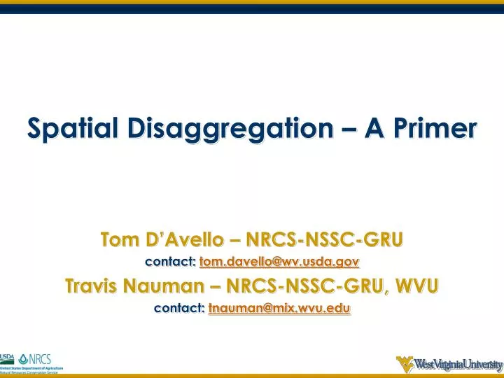
Spatial Disaggregation – A Primer. Tom D’Avello – NRCS-NSSC-GRU c ontact: tom.davello@wv.usda.gov Travis Nauman – NRCS-NSSC-GRU, WVU c ontact: tnauman@mix.wvu.edu. Overview. Define ‘Disaggregation’ Approaches and Tools West Virginia Illinois Arizona Summary

E N D
Spatial Disaggregation – A Primer Tom D’Avello – NRCS-NSSC-GRU contact: tom.davello@wv.usda.gov Travis Nauman – NRCS-NSSC-GRU, WVU contact: tnauman@mix.wvu.edu
Overview • Define ‘Disaggregation’ • Approaches and Tools • West Virginia • Illinois • Arizona • Summary • Literature list for your reference
What is spatial disaggregation? • The next opportunity for the NCSS • Add value to SSURGO • “The process of separating an entity into component parts based on implicit spatial relationships or patterns” – (Moore, 2008) • Getting more detail • Spatially refining maps to reflect the level of detail for current needs • Corresponding increased resolution of attributes • Trying to meet new types of demands
What is spatial disaggregation? • Mapping of components within map units • Usually complexes or associations for Order 2 & 3 soil surveys (SSURGO) • STATSGO2 effort • Alaska (Moore, 2008) • New needs served • modeling community • maintenance and improvement of the product is a primary charge of NCSS http://www.soilsurvey.org/tutorial/page1.asp
What is spatial disaggregation? • Ultimately, it is a refined segmentation of the landscape • Along with the spatial, the attributes are equally important • Map units have multiple parts with attributes • Example: Ponded parts of a larger map unit • Related to SDJR • Scope driven! • Area of Interest • Can be relevant to one, some or all map units.
Purpose of the demonstration • Demonstrate case studies across varying physiographic regions • Get feedback from soil scientists on their assessment of current soil maps • Investigate different digital techniques • Evaluate results • Develop materials and guidelines for application by soil scientists
West Virginia early efforts Component Soils Gilpin Craigsville Pineville Meckesville Laidig Cateache Shouns Guyandotte Dekalb SSURGO Map Units Gilpin-Laidig Pineville-Gilpin-Guyandotte Other
General disaggregation workflow • Goals • Scope • What data is accessible to help • Choose method • Implement • Validate Quality • (evaluate and iterate earlier steps as needed)
Current workflow in West Virginia • Goals • Soil series map on field scale grid • Scope • All map units in Pocahontas and Webster Counties, WV • What data is accessible to help • ~30-meter DEM (NED), Landsat Geocover (Fed. MDA, 2004), lithology, SSURGO • Choose method • SSURGO-derived expert rule training sets & classification tree ensemble (100 trees run on random subsets) • Implement • Run analysis with Access (SQL), GIS, and Python (or R) • Validate Quality • Independent pedons for ground truth
1. & 2. Goals and scope • Scope is key • define what needs to be disaggregated • Universal vs within map unit(s) (Local) • Local model (confined to existing map unit) • Keep original lines • Universal model • uses original survey to create but lines not used for final Local Universal Figures courtesy of Dave Hoover, NSSC
3. What data: SSURGO Legend Map Unit Inclusion Parent material Geomorphology Component Landscape attributes Components (not explicitly mapped) Horizon attributes Horizon Soil physical properties Soil chemical properties
3. What data: SSURGO • Most work done on SSURGO or equivalent scale maps • Raster (grids) used for modeling • to match environmental data West Virginia data
3. What data: environmental • Raster grids • Sometimes other polygon layers converted (e.g. geology) • Characterize variation within polygons using data that infer soil forming factors SSURGO lines over Landsat SSURGO lines over DEM SSURGO lines over landforms (Schmidt & Hewitt, 2004) Examples from West Virginia
4. Method: model techniques • Training Data • Match environmental data to components of interest • Use representative areas or pedon locations • Model Types • Expert landscape rules • Hardened or fuzzy • Statistical models • Area to Point Interpolations (Goovaerts, 2011) Dekalb series training areas in WV Example Classification Tree Model
5. & 6. Implement & Validate • Create raster disaggregation map • Validate with ground truth data • Different methods available WV example: universal model for Webster and Pocahontas Counties
Historical survey of Webster County, WV These folks were pretty good Milton Whitney Curtis Marbut Hugh Bennett Nice map, too!
Peoria, Illinois investigation • Goals • Components or phases within Sable and Ipava units • Scope • All Sable and Ipava map units within Peoria County • What data is accessible to help • 3-meter DEM (NED), SSURGO • Choose method • Expert rule training sets & classification trees • Implement • Run analysis with R, ArcGIS and ArcSIE • Validate Quality • Local soil scientist review.
Peoria, Illinois investigation1. Goals • Identification of Non-ponded and ponded phases in Sable units • Identification of poorly drained components in Ipava units
Peoria, Illinois investigation2. Scope - study site The project area is within MLRAs 95B, 108A, 108B, 108C and 115C ~900,000 acres of Sable ~1,186,000 acres of Ipava • Why here? • Availability of high resolution DEMs • Representative setting for Sable and Ipava • Good test for developing procedures to complete for entire extent of units when LiDAR coverage is complete
General setting2. Scope - study site Typical cross-section and qualitative description of Sable and Ipava soils
Variables developed3. Data - all derived from 3m DEM with ArcGIS/ArcSIE/SAGA GIS • Altitude above channel network • Curvature at numerous neighborhoods • Horizontal distance to flow channel • Maximum curvature –numerous neighborhoods • Minimum curvature –numerous neighborhoods • Multi-resolution ridge top flatness index • Multi-resolution valley bottom flatness index • Profile curvature –numerous neighborhoods • Relative position-numerous neighborhoods • Sink depth and Depression cost surface • Slope • Tangential curvature –numerous neighborhoods • Topographic position index • Vertical distance to flow channel • Wetness index
Exploratory Data Analysis4. Method • An extensive sample with soil series as a response was developed • Classification Tree in R to determine explanatory variables
Purpose of evaluation4. Method • Spatial data needs to be the driver for modeling effort • Efficient determination of explanatory variables • Efficient determination of thresholds for variables • Practical tools are needed to assist soil scientists in this effort
Results from classification tree5. Implement • Altitude above channel network • Horizontal distance to channel • Minimum curvature 120m neighborhood • Multi-resolution ridge top flatness index • Profile curvature 150m neighborhood • Relative position 90m neighborhood • Relative position 60m neighborhood • Relative position 30m neighborhood • Sink Depth • Slope 30m neighborhood • Topographic position index • Wetness index Input variables Important variables • Altitude above channel network • Relative Elevation (aka Relative position) • Sink Depth Developed 20+ datasets – 12 showed promise from qualitative review – 3 were identified through classification tree as explanatory variables in this example
Results from classification tree 5. Implement -Ipavaand Sable independently
Results from classification tree 5. Implement – walk through the splits Altitude above channel network >= 0.25 < 0.25
Results from classification tree 5. Implement – walk through the splits Relative position >= 0.595 < 0.595
Results from classification tree 5. Implement – walk through the splits Sink depth >= 1.472 < 1.472
Results from classification tree 5. Implement - Results of rules applied for Sable and Ipava
Results from classification tree • 5. Implement Rule base compared with SSURGO for Sable
Ponded vs. non-ponded Sable6. Validate Local - using depression depth Blue – likely depression/ponded Red -Yellow – no depression
Ponded vs. non-ponded Sable6. Validate Local - using depression cost surface Blue – likely depression/ponded Red -Yellow – no depression
Ponded vs. non-ponded Sable6. Validate Local - using 3m USGS NED • Zonal statistics indicate 41% of the area mapped as Sable is ponded • Based on selected thresholds • Verification and tuning of threshold values is ongoing
Ponded vs. non-ponded Sable 6. Validation/Data Local - using 10m USGS NED • Zonal statistics indicate 17% of the area is ponded Bigger legend Area “missed” with coarser 10m DEM
Ponded vs. non-ponded Ipava6. Validate Local - using 3m USGS NED • Zonal statistics indicate 9% of the area is ponded
Future effort for Peoria County • Populate component table - based on verified and validated thresholds • Rename map unit phases if needed • What is reasonable to improve product? • Accept line work and split components within existing map units? - A working copy in preparation for phase II of data recorrelation makes this feasible
Arizona – arid example • Goal • match environmental classification of soil forming factor raster layers to soil types. • Scope • Entire soil survey: Organ Pipe Cactus National Monument (ORPI) • Data • Used DEM and ASTER imagery to represent topography, vegetation, and geology • Method • Unsupervised classification (clustering) • Implement • Erdas Imagine and ArcGIS • Validate (evaluation) • Contingency tables (Chi2 Cramer’s V) to MUs; found separation of components in most complexes in field recon. (Nauman, 2009)
Arizona • More methods trials are planned for northeast AZ • Initial spatial data is being compiled • Model runs by late 2013
Summary • Disaggregation is a process that is defined by a need for more detail • Needs a directed scope • Tremendous amount of new data and computing abilities to incorporate • Disaggregating classic soil surveys • improves the detail of final maps without loss of accuracy and with no new data • more realistic representation of soil distribution (continuous – background probabilities) • Can use new field data in future to re-model for easy update (doing this in WV)
Next Steps • Match disaggregated data to ESDs • Further disaggregate to ESD state and transition models • Would better match imagery because management (e.g. pasture vs forest) is more easily detected with remote sensing. • Could map at state and/or community level for direct use in conservation planning • National Range and Pasture Handbook, 2003 • Currently submitting article for peer review documenting WV case study • Nauman, T., J.A. Thompson. (In prep). Semi-Automated Disaggregation of Conventional Soil Maps using Knowledge Driven Data Mining and Classification Trees
Resources – Available TrainingNRCS offers the following courses which provide an introduction to some of these techniques – check AgLearn • Spatial Analysis workshop (distance learning) • Introduction to Digital Soil Mapping (distance learning) • Digital Soil Mapping with ArcSIE (conventional class) • Remote Sensing for Soil Survey Applications (conventional class)
Literature Bui, E., B. Henderson, and K. Viergever. 2009. Using knowledge discovery with data mining from the Australian Soil Resource Information System database to inform soil carbon mapping in Australia. Global Biogeochemical Cycles 23. Bui, E.N. and Moran, C.J., 2001. Disaggregation of polygons of surficial geology and soil maps using spatial modelling and legacy data. Geoderma, 103(1-2): 79-94. Bui, E.N., A. Loughhead, and R. Corner. 1999. Extracting soil-landscape rules from previous soil surveys. Australian Journal of Soil Research 37:495-508. de Bruin, S., Wielemaker, W.G. and Molenaar, M., 1999. Formalisation of soil-landscape knowledge through interactive hierarchical disaggregation. Geoderma, 91(1–2): 151-172. Goovaerts, P., 2011. A coherent geostatistical approach for combining choropleth map and field data in the spatial interpolation of soil properties. European Journal of Soil Science, 62(3): 371-380. Häring, T., Dietz, E., Osenstetter, S., Koschitzki, T. and Schröder, B., 2012. Spatial disaggregation of complex soil map units: A decision-tree based approach in Bavarian forest soils. Geoderma, 185–186(0): 37-47. Kerry, R., Goovaerts, P., Rawlins, B.G. and Marchant, B.P., 2012. Disaggregation of legacy soil data using area to point kriging for mapping soil organic carbon at the regional scale. Geoderma, 170: 347-358. Li, S., MacMillan, R. A., Lobb, D. A., McConkey, B. G., Moulin, A., & Fraser, W. R. 2011. Lidar DEM error analyses and topographic depression identification in a hummocky landscape in the prairie region of Canada. Geomorphology, 129(3), 263-275. McBratney, A.B., 1998. Some considerations on methods for spatially aggregating and disaggregating soil information. Nutrient Cycling in Agroecosystems, 50(1-3): 51-62. MDA, Federal. 2004. Landsat Geocover TM 1990 & ETM+ 2000 Edition Mosaics Tile N-17-35 TM-EarthSat-MrSID. USGS, Sioux Falls, South Dakota.
Literature Moore, A. 2008. Spatial Disaggregation Techniques for Visualizing and Evaluating Map Unit Composition. NRCS 2008 National State Soil Scientist’s Workshop. Florence, Kentucky. ftp://ftp-fc.sc.egov.usda.gov/NSSC/NCSS/Conferences/state/2008/moore.pdf Nauman, T.W., 2009. Digital Soil-Landscape Classification for Soil Survey using ASTER Satellite and Digital Elevation Data in Organ Pipe Cactus National Monument, Arizona. MS Thesis. The University of Arizona. Nauman, T., J.A. Thompson, N. Odgers, and Z. Libohova. 2012. Fuzzy Disaggregation of Conventional Soil Maps using Database Knowledge Extraction to Produce Soil Property Maps, In B. Minasny, et al., (eds.) Digital Soil Assessments and Beyond: 5th Global Workshop on Digital Soil Mapping, Sydney, Australia. Schmidt, J. and Hewitt, A., 2004. Fuzzy land element classification from DTMs based on geometry and terrain position. Geoderma, 121(3-4): 243-256. Thompson, J.A. et al., 2010. Regional Approach to Soil Property Mapping using Legacy Data and Spatial Disaggregation Techniques, 19th World Congress of Soil Science, Soil Solutions for a Changing World, Brisbane, Australia. Wei, S. et al., 2010. Digital Harmonisation of Adjacent Soil Survey areas - 4 Iowa Counties, 19th World Congress of Soil Science, Soils Solutions for a Changing World, Brisbane, Australia. Wielemaker, W.G., de Bruin, S., Epema, G.F. and Veldkamp, A., 2001. Significance and application of the multi-hierarchical landsystem in soil mapping. Catena, 43(1): 15-34. Yang, L. et al., 2011. Updating Conventional Soil Maps through Digital Soil Mapping. Soil Science Society of America Journal, 75(3): 1044-1053. Zhu, A.X., 1997. A similarity model for representing soil spatial information. Geoderma, 77(2-4): 217-242. Zhu, A.X., Band, L., Vertessy, R. and Dutton, B., 1997. Derivation of soil properties using a soil land inference model (SoLIM). Soil Science Society of America Journal, 61(2): 523-533. Zhu, A.X., Band, L.E., Dutton, B. and Nimlos, T.J., 1996. Automated soil inference under fuzzy logic. Ecological Modelling, 90(2): 123-145.