Download
1 / 12
190 likes | 240 Views
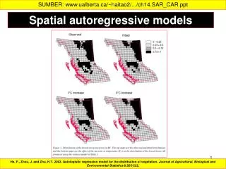
Spatial autoregressive methods. Nr245 Austin Troy Based on Spatial Analysis by Fortin and Dale, Chapter 5. Autcorrelation types. None: independence Spatial independence, functional dependence True autocorrelation>> inherent autoregressive Functional autocorr>> induced autoregressive.

E N D
Spatial autoregressive methods Nr245 Austin Troy Based on Spatial Analysis by Fortin and Dale, Chapter 5
Autcorrelation types • None: independence • Spatial independence, functional dependence • True autocorrelation>> inherent autoregressive • Functional autocorr>> induced autoregressive
Autocorrelation types • Double autoregressive • Notice there are now two autocorrelation parameters r-x and r-z
Effects? • Standard test statistics become “too liberal”—more significant results than the data justify • Because observations are not totally independent have lower actual degrees of freedom, or lower “effective sample size”: n’ instead of n; since t stat denominator = s/n, if n is too big it inflates the t statistic
What to do? Non-effective • Why not just adjust up the significance level? E.g. 99% instead of 95%? Because don’t how by how much to adjust without further information. Could end up with a test that is way too conservative • Why not just adjust sampling to only include “independent samples?” Because wasteful of data and because easy to mistake “critical distance to independence”
Best approach: Adjust effective sample size • For large sample sizes • So for instance n=1000 and ro=.4 means n’=429 • Problem is that, to be useful, autoregressive model (ro parameter) has to be an effective descriptor of the structure of autocorrelation of the data
Moving average models • How calculated depends on “order” • A simple model for adjusting sample size: first order autoregressive model, only immediate (first order) neighbors are correlated with ro>0. All other pairs are zero. • In such a model xi is a function of xi+1 and xi-1 • Hence half the info for xi is in each neighbor; produce ro=.5 for large n and n’=n/2. • An n order model can take form • Translates into generalized matrix form • With variance covariance matrix
Moving average • When you increase the order, calculating sample size gets complicated; e.g. second order model, where two ro parameters now • Important point: If there are several different levels of autocorrelation (rk), each rk must be incorporated even if non-significant; this can have a huge impact on the calculation of effective sample size • Fortin and Dale recommend not using moving average approach because very sensitive to irregularities in the data and can produce a wide range of estimates
Two dimensional approaches • Problem with MA approach as it was just presented is assumes one-dimensionality • In spatial data, xi depends on all neighbors most likely • Two best ways for dealing with this: • Simultaneous autoregressive models (SAR) • Conditional autoregressive models (CAR)
SAR • Based on concept of set of simultaneous equations to be solved. In this xi and xi-1 are each defined by their own equations • Where x is a vector and is linearly dependent on a vector of underlying variables z1,z2z3…. Given as matrix Z, u is a vector non-independent error terms with mean zero and var-covar matrix C • Spatial autocorrelation enters via u where • Here e is independent error term and W is neighbor weights standardized to row totals of 1. W is not necessarily symmetrical, allowing for inclusion of anisotropy.Wijis >0 if values at location i is not independent of value at location j
SAR • This yields the model • With variance covariance matrix (from u) • Note how similar to MA—difference is no inverse in formula • The elements of C are variances From Fortin and Dale p. 231
CAR • More commonly used in spatial statistics • Not based on spatial dependence per se; instead probability of a certain value is conditional on neighbor values • Similar to SAR, but requires that weight matrix be symmetrical • Here Where j is the autocorrelation parameter and V is a symmetrical weight matrix Any SAR process is a CAR process if V= W + WT – W TW