Download

1 / 63
790 likes | 1.65k Views
Spatial Clustering Methods. In Data Mining GDM. Ronald Treur. 23 September 2003. Contents. Spatial Clustering Considerations Clustering Algorithms Partitioning Methods Hierarchical Methods Density-based Methods Grid-based Methods Constraint-based Analysis Conclusion.

E N D
Spatial Clustering Methods In Data Mining GDM Ronald Treur 23 September 2003
Contents • Spatial Clustering • Considerations • Clustering Algorithms • Partitioning Methods • Hierarchical Methods • Density-based Methods • Grid-based Methods • Constraint-based Analysis • Conclusion
Spatial Clustering • Spatial clustering is the process of grouping a set of objects into classes or clusters so that objects within a cluster have high similarity in comparison to another but are dissimilar to objects in other clusters.
Considerations Cluster analyses has been studied for many years, as a branch of statistics In order to choose a clustering algorithm that is suitable for a particular application, many factors have to be considered. These include: • Application goal, quality vs speed and characteristics of the data
1. Application Goal • Example: Discovering good locations for setting up stores • A supermarket chain might like to cluster their customers such that the sum of the distance to the cluster centre is minimized (k-means, k-medoids).
1. Application Goal • Example: Image recognition & raster data analysis • Find natural clusters, clusters which are perceived as crowded together by the human eye (density-based)
2. Quality versus Speed A suitable clustering algorithm for an application must satisfy both the quality and speed requirements • Size of data (compression -> lossy) • Good quality, might be unable to handle large datasets
3. Characteristics of the Data • Types of data attributes: The similarity between two data objects is judged by the difference in their data attributes • When these are numeric: Euclidian & Manhattan distances can be computed • Binary, categorical and ordinal values make things much more complicated
3. Characteristics of the Data • Dimensionality: The dimensionality of the data refers to the number of attributes in a data object Many clustering algorithms which work well on low-dimensional data degenerate when the number of dimensions increase • Increase in running time • Decrease in cluster quality
3. Characteristics of the Data • Amount of noise in data: Some clustering algorithms are very sensitive to noise and outliers, a careful choice must be made if the data in the application contains a large amount of noise
Clustering Algorithms Four general categories: • Partitioning method • Hierarchical method • Density-based method • Grid-based method
Partitioning Methods Partitioning algorithms had long been popular clustering algorithms before the emergence of data-mining • k-means method • k-medoids method • Expectation maximization (EM)
Partitioning Algorithm Algorithm: The generalized iterative relocation algorithm Input: The number of clusters k and a database containing n objects Output: A set of k clusters which minimize a criterion function E 1. arbitrarily choose k centres/distributions as the initial solution 2. repeat • (re)compute membership of the objects according to present solution • update some/all clusters centres/distribution according to new memberships of the objects 5. until (no change to E)
The k-means method • Uses the mean value of the objects in a cluster as the cluster centre • E = ΣΣ|x-mi|2 where x is the point in space representing the given object and mi is the mean of cluster Ci • Relatively scalable and efficient in processing large data sets because the computational complexity of the algorithm is O(nkt)
The k-means method • In step 3 of the algorithm, k-means assigns each object to its nearest centre, forming a new set of clusters • In step 4, all the centres of these new clusters are then computed by taking the mean of all the objects in each cluster • This is repeated until the criterion function E does not change after an iteration
Partitioning Algorithm - k means Algorithm: The generalised iterative relocation algorithm Input: The number of clusters k and a database containing n objects Output: A set of k clusters which minimize a criterion function E 1. arbitrarily choose k centres/distributions as the initial solution 2. repeat • assign each object to its nearest cluster • compute all the centers of the clusters according to new memberships of the objects 5. until (no change to E)
The k-medoids method • Unlike the k-means and EM algorithm, the k-medoids method uses the most centrally located object (medoids) in a cluster to be the cluster centre • Like k-means, objects are assigned to its nearest centre • Less sensitive to noise and outliers • Higher running time
The k-medoids method • Initialisation: k objects are randomly selected to be cluster centres • Step 3 is not used since this step is already handled in step 4 of the algorithm • At most one centre will be changed in step 4 for each iteration • This change must result in a decrease in the criterion function
The k-medoids method • Replaces one medoid with one non-medoid as long as the quality of the resulting clustering is improving • Replacement medoids are selected randomly • Use Partitioning Around Medoids (PAM) • CLARA and CLARANS are methods to handle larger data
Expectation Maximization Instead of representing each cluster using a single point, the EM algorithm represents each cluster using a probability distribution. A d-dimensional Gaussian distribution representing a cluster Ci is parameterized by the mean of the cluster ui, and a d x d covariance matrix Mi
Hierarchical Methods Create a hierarchical decomposition of the given set of data objects forming a dendrogram - a tree which splits the database recursively into smaller subsets The dendrogram can be formed “bottom-up” (agglomerative) and “top-down” (divisive)
Hierarchical Methods • Early methods: AGlomerative NESting (AGNES) and DIvisia ANAlysis (DIANA) often result in erroneous clusters • More recent methods, CURE and CHAMELEON utilizes a more complex principle. Less errors are made • Other approaches refine results afterwards using iterative relocation
AGNES and DIANA • AGENS: Bottom-up, start by placing each object in a single cluster and then merge these into larger and larger clusters untill all objects are in a single cluster • DIANA: Top-down, the exact reverse of Bottom-up. Start with a single cluster and break it down
AGNES and DIANA • The algorithms are simple and often encounter difficulties regarding the selection of merge and split points. Such a decision is critical because once a group of objects is merged or split, the process at the next step will operate on the newly generated clusters • Do not scale well
BIRCH Balanced Iterative Reducing and Clustering using Hierarchies • Compress data into many small subclusters • Perform clustering on subclusters • Due to compression, clustering can be performed in main memory and the algorithm only needs to scan the database once
CURE Clustering Using REpresentatives • Like AGNES but uses a much more sophisticated principle when merging clusters • Instead of a single centroid, a fixed number of well-scattered objects are selected to represent each cluster • The selected representative objects are shrunk towards there their cluster centres
CHAMELEON • Similar to CURE, but • Two clusters will be merged if the inter-connectivity and closeness of the merged cluster is very similar to the inter-connectivity and closeness of the two individual clusters before merging
CHAMELEON • To form initial subclusters, first create a graph G = (V,E) where each node vεV represents a data object, and a weighted edge (vi, vj) exists between two nodes vi and vj, if vj is one of the k-nearest neighbours of vi • The weight of each edge in G represents the closeness between the two data objects it connects
CHAMELEON • Use graph partitioning algorithm to recursively partition G into many small unconnected subgraphs by doing a min-cut on G at each level of recursion • min-cut: partitioning of G into roughly two parts of equal size such that the total weight of the edges being cut is minimized
CHAMELEON • It has been shown that CHAMELEON is more effective than CURE • The processing cost for high-dimensional data may require O(n2) time for n objects in the worst case
Density-based Methods Cluster methods that are based on a distance measure between objects have certain difficulties finding clusters with arbitrary shapes Density method: Regard clusters as dense regions of objects in the data space which are separated by regions of low density Density based methods can be used to filter out noise
DBSCAN • Density-based clustering algorithm that grows regions with sufficiently high density into clusters • Requires two parameters ε and Minpts • The neighbourhood within a radius ε of a given object is called the ε-neighbourhood • An object with at least Minpts of objects within its ε-neighbourhood is called a core object
DBSCAN • The clustering follows the following rules: • An object can belong to a cluster if and only if it lies within the ε-neighbourhood of some core object in the cluster • A core object o within the ε-neighbourhood of another core object p must belong to the same cluster as p • A non-core object q within the ε-neighbourhood of some core objects p1,..pi, i > 0 must belong to the same cluster as at least one of the core objects p1,..pi • A non-core object r which dows not lie within the ε-neighbourhood of any core object is considered to be noise
DENCLUE • Based on a set of density functions • Build on the following ideas: • The influence of each data point can be formally modeled using a mathematical function (influence function) which describes the impact of the data point within its neighbourhood
DENCLUE • Build on the following ideas: (cont.) • The overall density of the data space can be modeled as the sum of the influence functions of all data points • Clusters can then be determined mathematically by identifying density attractors, where the density attractors are local maxima of the overall density function
Grid-based Methods Density based methods like DBSCAN and OPTICS are index-based methods that face a breakdown in efficiency when the number of dimensions is high To enhance the efficiency of clustering, a grid-based clustering approach uses a grid data structure. It quantizes the space into a finite number of cells
Grid-based Methods • Main advantage: Its fast processing time which is typically independent of the number of data objects, but dependent on only the number of cells in each dimension in the quantized space • Examples: • STatistical INformation Grid (STING) • CLustering In QUEst (CLIQUE)
STING • Grid-based multiresolution data structure in which the spatial area is divided into rectangular cells • There are usually several levels of rectangular cells to correspond with different level of resolution. These form a hierarchical structure • Statistical information about the attributes in each grid cell (such as mean, maximum and minimum values) are precomputed and stored
STING • Statistical parameters of higher-level cells can be easily computed from the parameters of the lower-level cells. • These parameters include: • count (number of objects) • mean, standard deviation, minimum, maximum • type of distribution the attribute value in the cell follows
STING • Data are loaded bottom-up, starting at the bottom-most level (the level with the highest resolution) • To perform clustering users must supply the density-level as an input parameter • Using this parameter a top-down, grid-based method is used to find regions with sufficient density by adopting the following procedure:
STING • A layer within the hierarchical structure is determined from which the query-answering process is to start. This layer typically contains a small number of cells. • For each cell in the current layer we compute the confidence interval that the cell will be relevant to the result of the clustering. Cells that do not meet the confidence level will be removed from further consideration
STING • The relevant cells are then refined to finer solutions by repeating this procedure at the next level of the structure. • This process is repeated until the bottom layer is reached. At this time, if the query specification is met, the regions of relevant cells that satisfy the query are returned. Otherwise, the data that fall into the relevant cells are retrieved, and further processed until they meet the requirements
STING • Advantages of STING: • The grid-based computation is query-independent since statistical information stored in each cell represents summary information, independent of the query • The grid structure facilitates parallel processing and incremental updating • The method is very efficient
STING • Disadvantages of STING: • The quality depends on the granularity of the lowest level. If it is very fine, the cost of processing will increase; however if it is to coarse it may reduce the quality of cluster analysis • It does not consider spatial relationship between children and their neighbouring cells for construction of the parent cell
WaveCluster Multiresolution clustering algorithm that first summarizes the data by imposing a multidimensional grid structure on the data space. It the uses a wavelet transformation to transform the original feature space, finding dense region in the transformed space