Download
1 / 25
250 likes | 397 Views
Semi-implicit predictor-corrector methods for atmospheric models. Colm Clancy Janusz A. Pudykiewicz Atmospheric Numerical Weather Prediction Research, Environment Canada PDEs on the Sphere, 26 th of September 2012. Motivation.

E N D
Semi-implicit predictor-corrector methods for atmospheric models Colm Clancy Janusz A. Pudykiewicz Atmospheric Numerical Weather Prediction Research, Environment Canada PDEs on the Sphere, 26th of September 2012
Motivation • Development of a finite-volume atmospheric model on an icosahedral grid (Pudykiewicz 2006, 2011) • Investigation of stable time integration schemes, beyond the traditional semi-implicit leapfrog • Some recent work: Williams (2011), Durran & Blossey (2012), Kar (2012)
General ODE system ‘Traditional’ semi-implicit, (SILF):
Semi-implicit predictor-corrector approach Predictor stage, for : Corrector stage, for :
Implicit linear terms: Trapezoidal AM2*
Many possible combinations… Examples:
Shallow water tests • Shallow water model of Pudykiewicz (2011) • Iterative GCR(4) solver for Helmholtz equations (Smolarkiewicz and Margolin, 2000) • No explicit diffusion • Filter of Williams (2011) for the semi-implicit leapfrog • Spatial resolution: grid 6 (40,962 nodes, ~112km).Reference: grid 7 (163,842 nodes, ~56km) with RK4 at 90s time-step
Efficiency • Predictor-corrector schemes: two elliptic solver calls per time-step • Consider total number of iterations per step
Conclusions and further work • Semi-implicit predictor-corrector schemes offer an accurate alternative to the traditional leapfrog: • Stable • No time filter necessary • Efficiency not affected • Future tests with a three-dimensional baroclinic model • Comparison with other time integration methods
References • Clancy & Pudykiewicz (2012); to appear in J. Comp. Phys. • Durran & Blossey (2012); Mon. Weather. Rev. 140, 1307-1325 • Kar (2012); Mon. Weather. Rev. 134, 2916-2926 • Pudykiewicz (2006); J. Comp. Phys. 213, 358-390 • Pudykiewicz (2011); J. Comp. Phys. 230, 1956-1991 • Smolarkiewicz & Margolin (2000). Proc. ECWMF Workshop, 5-7 June 2000, 137-159 • Williams (2011); Mon. Weather. Rev. 139, 1996-2007 • Williamson et al. (1992); J. Comp. Phys. 102, 211-224