Download
1 / 24
400 likes | 1.44k Views
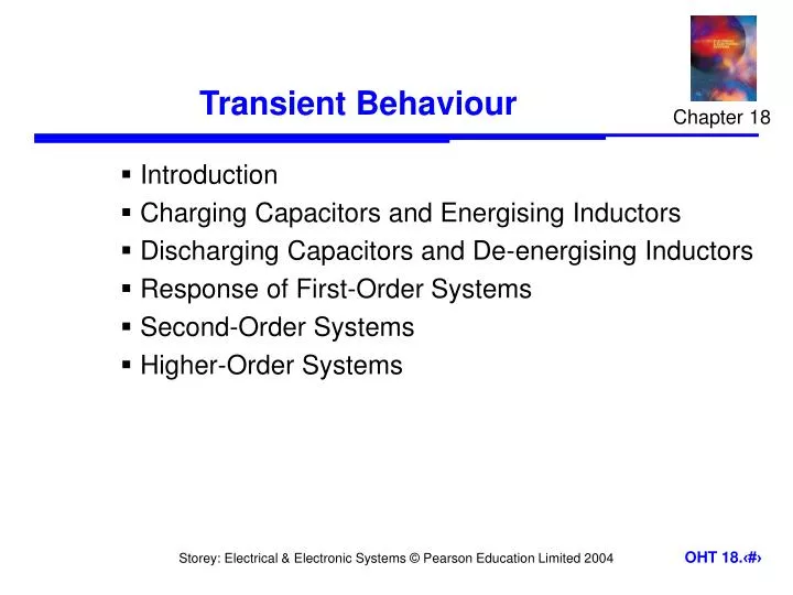
Chapter 18. Transient Behaviour. Introduction Charging Capacitors and Energising Inductors Discharging Capacitors and De-energising Inductors Response of First-Order Systems Second-Order Systems Higher-Order Systems. 18.1. Introduction.

E N D
Chapter 18 Transient Behaviour • Introduction • Charging Capacitors and Energising Inductors • Discharging Capacitors and De-energising Inductors • Response of First-Order Systems • Second-Order Systems • Higher-Order Systems
18.1 Introduction • So far we have looked at the behaviour of systems in response to: • fixed DC signals • constant AC signals • We now turn our attention to the operation of circuits before they reach steady-state conditions • this is referred to as the transient response • We will begin by looking at simple RC and RL circuits
18.2 Charging Capacitors and Energising Inductors Capacitor Charging • Consider the circuit shown here • Applying Kirchhoff’s voltage law • Now, in a capacitor • which substituting gives
The above is a first-order differential equation with constant coefficients • Assuming VC = 0 at t = 0, this can be solved to give • see Section 18.2.1 of the course text for this analysis • Since i = Cdv/dt this gives (assuming VC = 0 at t = 0) • where I = V/R
Inductor energising • A similar analysis of this circuit gives where I = V/R – see Section 18.2.2 for this analysis
Thus, again, both the voltage and current have an exponential form
18.3 Discharging Capacitors and De-energising Inductors Capacitor discharging • Consider this circuit for discharging a capacitor • At t = 0, VC = V • From Kirchhoff’s voltage law • giving
Solving this as before gives • where I = V/R – see Section 18.3.1 for this analysis
In this case, both the voltage and the current take the form of decaying exponentials
Inductor de-energising • A similar analysis of thiscircuit gives • where I = V/R – see Section 18.3.1for this analysis
And once again, both the voltage and the current take the form of decaying exponentials
18.4 Response of First-Order Systems • Initial and final value formulae • increasing or decreasing exponential waveforms (for either voltage or current) are given by: • where Viand Ii are the initial values of the voltage and current • where Vfand If are the final values of the voltage and current • the first term in each case is the steady-state response • the second term represents the transient response • the combination gives the total response of the arrangement
Example – see Example 18.3 from course text The input voltage to the following CR network undergoes a step change from 5 V to 10 V at time t = 0. Derive an expression for the resulting output voltage.
Here the initial value is 5 V and the final value is 10 V. The time constant of the circuit equals CR = 10 103 20 10-6 = 0.2s. Therefore, from above, for t 0
Response of first-ordersystems to a squarewaveform • see Section 18.4.3
Response of first-ordersystems to a squarewaveform of differentfrequencies • see Section 18.4.3
18.5 Second-Order Systems • Circuits containing both capacitance and inductance are normally described by second-order differential equations. These are termed second-order systems • for example, this circuit is described by the equation
When a step input is applied to a second-order system, the form of the resultant transient depends on the relative magnitudes of the coefficients of its differential equation. The general form of the response is • where n is the undamped natural frequency in rad/s and (Greek Zeta) is the damping factor
Response of second-order systems =0 undamped <1 under damped =1 critically damped >1 over damped
18.6 Higher-Order Systems • Higher-order systems are those that are described by third-order or higher-order equations • These often have a transient response similar to that of the second-order systems described earlier • Because of the complexity of the mathematics involved, they will not be discussed further here
Key Points • The charging or discharging of a capacitor, and the energising and de-energising of an inductor, are each associated with exponential voltage and current waveforms • Circuits that contain resistance, and either capacitance or inductance, are termed first-order systems • The increasing or decreasing exponential waveforms of first-order systems can be described by the initial and final value formulae • Circuits that contain both capacitance and inductance are usually second-order systems. These are characterised by their undamped natural frequency and their damping factor