Download
1 / 55
780 likes | 1.66k Views
Make to Stock (MTS) vs. Make to Order (MTO). Made-to-stock (MTS) operations Product is manufactured and stocked in advance of demand. Inventory permits economies of scale and protects against stockouts due to variability of interarrival time and processing time.

E N D
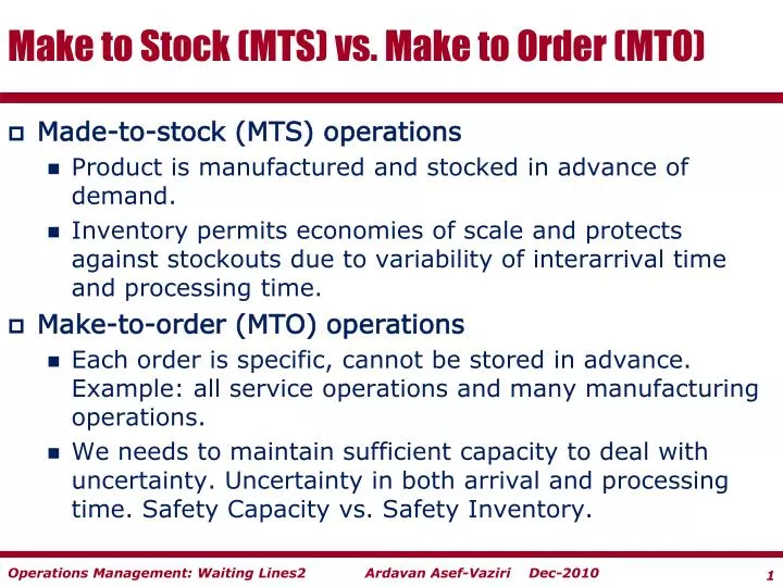
Make to Stock (MTS) vs. Make to Order (MTO) • Made-to-stock (MTS) operations • Product is manufactured and stocked in advance of demand. • Inventory permits economies of scale and protects against stockouts due to variability of interarrival time and processing time. • Make-to-order (MTO) operations • Each order is specific, cannot be stored in advance. Example: all service operations and many manufacturing operations. • We needs to maintain sufficient capacity to deal with uncertainty. Uncertainty in both arrival and processing time. Safety Capacity vs. Safety Inventory.
MTO Examples • Banks (tellers, ATMs, drive-ins). • Fast food restaurants (counters, drive-ins). • Retail (checkout counters). • Airline (reservation, check-in, takeoff, landing, baggage claim). • Hospitals (ER, OR, HMO). • Service facilities (repair, job shop, ships/trucks load/unload). • Call centres (telemarketing, help desks, 911 emergency) • More and more production systems now follow Dell computer operations model.
Article: The Psychology of Waiting Lines • Unoccupied time feels longer than occupied time. • Pre-process waits feels longer than in-process waits. • Anxiety makes waits seem longer. • Uncertain waits are longer than known, finite waits. • Unexplained waits are longer than explained waits. • Unfair waits are longer than equitable waits. • The more valuable the service, the longer I will wait. • Solo waiting feels longer than group waiting.
A Call Centre The Call Centre Process Sales Reps Processing Calls (Service Process) Incoming Calls (Customer Arrivals) Answered Calls (Customer Departures) Calls on Hold (Service Inventory) Blocked Calls (Due to busy signal) Abandoned Calls (Due to long waits) Calls In Process (Due to long waits)
Characteristics of Waiting Lines (Queuing Systems) • The time of the arrival of an order is not known ahead of time. It is a random variable with estimated mean and standard deviation. • The time of the next telephone call is not known. • The service time is not known (precisely) ahead of time. It is a random variable with estimated mean and standard deviation. • The time a customers spends on the web page of amazon.com is not precisely known. • The time a customer spends speaking with the teller in the bank is unknown
AVERAGE Processing Time TpAVERAGE Processing Rate Rp Tp : Processing time. Tp units of time. Ex. on average it takes 5 minutes to serve a customer. Rp : processing rate. Rp flow units are handled per unit of time. If Tp is 5 minutes. Compute Rp. Rp= 1/5 per minute, or 60/5 = 12 per hour.
More than One Server; c Servers Tp : processing time. Rp : processing rate. What is the relationship between Rp and Tp? If we have one resource Rp= 1/Tp • What is the relationship between Rp and Tp when we have more than one resource; We have c recourses Rp= c/Tp Each customer always spends Tp unites of time with the server
Average Processing Rate of c Servers Tp= 5 minutes. Processing time is 5 minute. Each customer on average is with the server for 5 minutes. c = 3, we have three servers. Processing rate of each server is 1/5 customers per minute, or 12 customer per hour. Rp is the processing rate of all three servers. Rp = c/Tp Rp= 3/5 customers/minute, or 36 customers/hour.
Inter-arrival Time (Ta) and Arrival Rate (Ri) Ta:customer inter-arrival time. On average each 10 minutes one customer arrives. Ra:customer arrival (inflow) rate. What is the relationship between Ta and Ri Ta = every ten minutes one customer arrives How many customers in a minute? 1/10; Ra= 1/Ta= 1/10 Ri = 1/10 customers per min; 6 customers per hour Ra= 1/Ta
Throughput = Min (Ri,Rp) Ra MUST ALWAYS <= Rp. We will show later that even Ra=Rp is not possible. Incoming rate must be less than processing rate. Throughput = Flow Rate R= Min (Ra, Rp) . Stable Process = Ra< Rp,, so that R= Ra Safety Capacity Rs = Rp– Ra
Buffer (waiting line) and Processors (Servers) What is the waiting time in the servers (processors)? Throughput? Flow time T = Ti+ Tp Inventory I = Ii + Ip Ti: waiting time in the inflow buffer Ii: number of customers in the inflow buffer
Utilization is Always Less than 1 = Utilization = inflow rate / processing rate = throughout / process capacity = R/ Rp < 1 Safety Capacity = Rp– R For example , R = 6 per hour, processing time for a single server is 6 min Rp= 12 per hour, =R/ Rp = 6/12 = 0.5 Safety Capacity = Rp– R = 12-6 = 6
Given the Utilization, How Many Flow Units are in the Processor(s) Given a single server. And a utilization of r = 0.5 How many flow units are in the server ? • Given 2 servers. And a utilization of r = 0.5 • How many flow units are in the servers ?
Characteristics of Queuing Systems • Variability in arrival time and service time leads to • Idleness of resources • Waiting time of customers (orders) to be processed • We are interested in evaluating two measures: • Average waiting time of flow units. Average waiting time in the waiting line and in the system (Waiting line + Processor). • Average number of flow units. The average number of orders (customers) waiting in the waiting line (to be then processed).
The Little’s Law Applies Everywhere R • Flow time T Ti+ Tp • Inventory I = Ii + Ip Ip= R Tp I = R T Ii = R Ti R = I/T = Ii/Ti = Ip/Tp Tp if 1 server Rp = 1/Tp In general, if c servers Rp = c/Tp
Operational Performance Measures From the Little’s Law R = Ip/Tp From definition of Rp Rp = c/Tp = R/ Rp= (Ip/Tp)/(c/Tp) = Ip/c And it is obvious that = Ip/c Because on average there are Ip people in the processors and the capacity of the servers is to serve c customers at a time. = R/Rp = Ip/c
Financial Performance Measures • Sales • Throughput Rate • Cost • Capacity utilization • Number in queue / in system • Customer service • Waiting Time in queue /in system
Utilization and Variability • Two key drivers of process performance are Utilization and Variability. • The higher the utilization the longer the waiting line. • High capacity utilization ρ= R/ Rp or low safety capacity Rs =R –Rp, due to • High inflow rate R • Low processing rate Rp=c / Tp, which may be due to small-scale c and/or slow speed 1 /Tp • The higher the variability, the longer the waiting line.
Drivers of Process Performance • Variability in the interarrival time and processing time can be measured using standard deviation. Higher standard deviation means greater variability. • Coefficient of Variation: the ratio of the standard deviation of interarrival time (or processing time) to the mean. • Ca = coefficient of variation for interarrival times • Cp = coefficient of variation for processing times
Operational Performance Measures Flow time T = Ti+ Tp Inventory I = Ii + Ip Ti: waiting time in the inflow buffer = ? Ii: number of customers waiting in the inflow buffer =?
Queuing Models EXACT Formulas • The exact formulas are rather complicated. • A set of excel sheet are provided at the end of this lecture. • We relay on the approximation formula, given shortly, and our understanding of the waiting line logics.
The Queue Length APPROXIMATION Formula • R/Rp,whereRp = c / Tp • Caand Cp are the Coefficients of Variation • Standard Deviation/Mean of the inter-arrival or processing times (assumed independent) Utilization effect U-part Variability effect V-part
Factors affecting Queue Length This part captures the capacity utilization effect. It shows that queue length increases rapidly as approaches 1. • This part captures the variability effect. It shows that the queue length increases as the variability in interarrival and processing times increases. • Even if the processing capacity is not fully utilized, whenever there is variability in arrival or in processing times, queues will build up and customers will have to wait.
Arrival Rate at an Airport Security Check Point What is the queue size? What is the capacity utilization?
Flow Times with Arrival Every 6 Secs What is the queue size? What is the capacity utilization?
Flow Times with Arrival Every 6 Secs What is the queue size? What is the capacity utilization?
Flow Times with Arrival Every 6 Secs What is the queue size? What is the capacity utilization?
Utilization – Variability - Delay Curve Average Time in System T Variability Increases Tp 100% r Utilization (ρ)
Lessons Learned • If inter-arrival and processing times are constant, queues will build up if and only if the arrival rate is greater than the processing rate. • If there is (unsynchronized) variability in inter-arrival and/or processing times, queues will build up even if the average arrival rate is less than the average processing rate. • If variability in interarrival and processing times can be synchronized (correlated), queues and waiting times will be reduced.
Terminology and Classification of Waiting Lines • Terminology: The characteristics of a queuing system is captured by five parameters: • Arrival pattern • Service pattern • Number of server • Restriction on queue capacity • The queue discipline
Terminology and Classification of Waiting Lines • M/M/1 • Exponential interarrival times • Exponential service times • There is one server. • No capacity limit • M/G/12/23 • Exponential interarrival times • General service times • 12 servers • Queue capacity is 23
Example; Coefficient of Variation of Interarrival Time A sample of 10 observations on Interarrival times in minutes 10,10,2,10,1,3,7,9, 2, 6 minutes. =AVERAGE () Avg. interarrival time = 6 min. Ra= 1/6 arrivals / min. =STDEV() Std. Deviation = 3.94 Ca 3.94/6 = 0.66 C2a= (0.66)2 =0.4312
Example: Coefficient of Variation of Processing Time A sample of 10 observations on Processing times in minutes 7,1,7 2,8,7,4,8,5, 1 minutes. Tp= 5 minutes Rp = 1/5 processes/min. Std. Deviation = 2.83 Cp = 2.83/5 = 0.57 C2p = (0.57)2 = 0.3204
Example: Utilization and Safety Capacity Ra=1/6 < RP =1/5 R = Ra = R/ RP = (1/6)/(1/5) = 0.83 With c = 1, the average number of passengers in queue is as follows: Ii = [(0.832)/(1-0.83)] ×[(0.662+0.572)/2] = 1.56 On average 1.56 passengers waiting in line, even though safety capacity is Rs= RP - Ra= 1/5 - 1/6 = 1/30 passenger per minute, or 2 per hour.
Example: Other Performance Measures Waiting time in the line? Ti=Ii/R = (1.56)(6) = 9.4 minutes. Waiting time in the system? T = Ti+Tp Since TP = 5 T = Ti + TP= 14.4 minutes Total number of passengers in the process is: I = RT = (1/6) (14.4) = 2.4 Alternatively, 1.56 in the buffer. How many in the process? I = 1.56 + 0.83 = 2. 39
Example: Now suppose we have two servers. Compute R, Rp and : Ta= 6 min, Tp = 5 min R = Ra= 1/6 per minute Processing rate for one processor 1/5 for 2 processors Rp = 2/5 = R/Rp = (1/6)/(2/5) = 5/12 = 0.417 On average 0.076 passengers waiting in line. safety capacity is Rs= RP - Ra= 2/5 - 1/6 = 7/30 passenger per minute, or 14 passengers per hour
Other Performance Measures for Two Servers Other performance measures: Ti=Ii/R = (0.076)(6) = 0.46 minutes Compute T? T = Ti+Tp Since TP = 5 T = Ti + TP= 0.46+5 = 5.46 minutes Total number of passengers in the process is: I= 0.08 in the buffer and 0.417 in the process. I = 0.076 + 2(0.417) = 0.91
Effect of Pooling Ra =R= 10/hour Tp= 5 minutes Interarrival time Poisson Service time exponential Ra/2 Server 1 Queue 1 Ra Ra/2 Server 2 Queue 2 Server 1 Ra Queue Server 2
Effect of Pooling : 2M/M/1 Ra/2 Server 1 Ra/2 = R= 5/hour Tp= 5 minutes C = 1 Rp = 12 / hour = 5/12 = 0.417 Queue 1 Ra Ra/2 Server 2 Queue 2
Comparison of 2M/M/1 with M/M/2 Ra/2 Server 1 Queue 1 Ra Ra/2 Server 2 Queue 2 Server 1 Ra Queue Server 2
Effect of Pooling: M/M/2 Ra=R= 10/hour Tp= 5 minutes C = 2 Rp = 24 /hour = 10/24 = 0.417 AS BEFORE for each processor Server 1 Ra Queue Server 2
Effect of Pooling • Under Design A, • We have Ra = 10/2 = 5 per hour, and TP= 5 minutes, c =1, we arrive at a total flow time of 8.6 minutes • Under Design B, • We have Ra =10 per hour, TP= 5 minutes, c=2, we arrive at a total flow time of 6.2 minutes • So why is Design B better than A? • Design A the waiting time of customer is dependent on the processing time of those ahead in the queue • Design B, the waiting time of customer is partially dependent on each preceding customer’s processing time • Combining queues reduces variability and leads to reduce waiting times
Performance Improvement Levers • Decrease variability in customer inter-arrival and processing times. • Decrease capacity utilization. • Synchronize available capacity with demand.
1. Variability Reduction Levers • Customers arrival are hard to control • Scheduling, reservations, appointments, etc…. • Variability in processing time • Increased training and standardization processes • Lower employee turnover rate more experienced work force • Limit product variety, increase commonality of parts
2. Capacity Utilization Levers • If the capacity utilization can be decreased, there will also be a decrease in delays and queues. • Since ρ=R/Rp, to decrease capacity utilization there are two options • Manage Arrivals: Decrease inflow rate Ra • Manage Capacity: Increase processing rate Rp • Managing Arrivals • Better scheduling, price differentials, alternative services • Managing Capacity • Increase scale of the process (the number of servers) • Increase speed of the process (lower processing time)
3. Synchronizing Capacity with Demand • Capacity Adjustment Strategies • Personnel shifts, cross training, flexible resources • Workforce planning & season variability • Synchronizing of inputs and outputs, Better scheduling