Download
1 / 10
130 likes | 361 Views
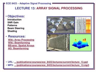
LECTURE 13: ARRAY SIGNAL PROCESSING. Objectives: Introduction SNR Gain Patterns Beam Steering Shading Resources: Wiki: Array Processing Wiki: Beamforming BEvans : Spatial Arrays AG: Beamforming. • URL: .../publications/courses/ece_8423/lectures/current/lecture_13.ppt

E N D
LECTURE 13: ARRAY SIGNAL PROCESSING • Objectives:IntroductionSNR GainPatternsBeam SteeringShading • Resources:Wiki: Array ProcessingWiki: BeamformingBEvans: Spatial ArraysAG: Beamforming • URL: .../publications/courses/ece_8423/lectures/current/lecture_13.ppt • MP3: .../publications/courses/ece_8423/lectures/current/lecture_13.mp3
Introduction • Array processing deals with applying signal processing techniques to a spatially distributed group of sensors. • The potential lies in achieving improvements in the SNR. • The spatial dimensions introduces the possibility of directional discrimination between the signal and the interference (e.g., noise). • The measured signals are often electromagnetic (e.g., deep space radio telescopes, radar) or acoustic (e.g., auditoriums, automobiles). • The arrays can be arranged in a number of topologies (1D, 2D, and even 3D). • Often, achieving an improvement in the SNR involves detecting and tracking the direction of the signal. • This is achieved by independent adjustment of the time delays associated with each sensor. The analysis is completely analogous to that for phased antenna arrays. • Adaptive signal processing is used to estimate and optimize the weights and delays associated with the sensors. • One big advantage of the “electronic approach” is the ability to track multiple targets from the same, fixed array (formerly done via rotating antennae).
Basic Array Properties • We will focus on arrays where the sensors are uniformly spaced. • Other configurations and spacing can be dealt with using an analysis that parallels sampling theory. • The output of the array is a linear combination of the inputs: • (The weights can be complex.) • Assume the transmission path is linear and time-invariant: • hj(t) represents the transfer function from the source to the sensor. It can be simple, such as a time delay dependent on the distance: • Denote interference as u(t) and noise as v(t).
SNR Gain By Summation • Suppose the signal is incident at broadside ( = 0) with wi= 1. • Assume each measurement is corrupted by vi(t) which is uncorrelated from sensor to sensor: • The input SNR may be defined by: • The array output is: • The output SNR is: • The gain in SNR (an upper bound) is linearly proportional to the number of sensors:
Sensitivity Patterns For A 2-Sensor Array • The sensitivity of the array can be show to be a function of the incident angle of the plane wave.
Beam Steering • Beam steering is the process ofrotating the main lobe of the arraypattern in the direction of the incoming signal. • This is done by simply delaying each sensor by an amount proportional to the time it takes for the signal to propagate a distance equal to the sensor spacing. • The angle of the main lobe obeys asimple relation: • The process of steering the beamusing time delay and summing thesignals is known as the delay andsum beamformer. • Note that this delay can be donedigitally as part of the beamsteering algorithm. Also, multiple beams can be managed simultaneously.
Array Shading (Deterministic) • Given N sensors, we can weight the sensor outputs to steer the array in the direction of a signal, AND to steer nulls in the direction of noise. • We will first explore a deterministic way of doing this using a priori information, and then later in this chapter explore ways to do this adaptively. • Define a narrowband signal: • where m(t) is an amplitude modulation which is considered slowly varying so that it can be assumed to be constant across the array. • Define a steering vector, s, associated with an angle : • where d is the sensor spacing, and k= /c. • Define a vector of measurements as: • For M separate sources:
Optimizing Weights • We can define an NxM matrix, Q, consisting of the steering vectors, and a vector of the modulated signals: • We can define a weight vector that we will use to steer the array: • We can apply a gain, g, to a signal from direction : • For M sources, we can have M distinct gains: • Assuming the signal is associated with the first sensor, we can steer nulls in the other directions by solving: • or, equivalently solving the matrix equation: • If the number of sources equals the number of sensors, Q is square, and we can solve this set. If the number of sources is less than the number of sensors, we need to add extra constraints.
Summary • Introduced array signal processing. • Demonstrated an upper bound on the gain that can be achieved. • Discussed basic properties of the array. • Derived a way to improve performance by steering the array in the direction of the signal and steering nulls in the direction of the interference. • Next: demonstrate how to do this adaptively. • Advantages: • No requirement on a priori information about the signal or interference. • Adapt to changes in the signal or the interference. • Adapt to noise. • Track multiple signals simultaneously.