Download
1 / 22
220 likes | 487 Views
Hurricane Initialization in HWRF model. Qingfu Liu, Naomi Surgi, Stephen Lord Vijay Tallapragada, Young Kwon, Robert Tuleya Zhan Zhang, Janna Oconnor Acknowledgement: Wan-Shu Wu John Derber Russ Treadon. HWRF analysis cycle. HWRF analysis at time t-6.

E N D
Hurricane Initialization in HWRF model Qingfu Liu, Naomi Surgi, Stephen Lord Vijay Tallapragada, Young Kwon, Robert Tuleya Zhan Zhang, Janna Oconnor Acknowledgement: Wan-Shu Wu John Derber Russ Treadon
HWRF analysis cycle HWRF analysis at time t-6 9 hours forecast at time t-3, t, t+3 Relocate hurricane vortex and modify its structure t t+6 Run GSI analysis at time t 126 hours forecast
Creation of the background fields • Large scale flow in HWRF analysis is worse compared to those from GFS analysis after many cycled runs • In current HWRF analysis, we replace the HWRF environmental flow with those from GFS analysis (this should change back in the future) • Hurricane vortex come from HWRF 6 hours forecast Background fields = Environment flow from GFS analysis + Modified HWRF forecasted hurricane vortex
The following background fields are created for the GSI data assimilation: 750x750 outer nest data 120x120 intermediate nest data (add a transition zone) • After GSI, the two domains are merged together Create 750x750 outer nest data and 60x60 inner nest data (Jim Purser provides the weighting function)
Correction of the Hurricanes (Storms) • correct the size of hurricane eyewall • correct wind components • compute new surface pressure and 3D temperature fields • correct moisture (hydrometeor) • correct storm depth (or middle to upper level structure)
1. Storm size correction • HWRF has tendency to increase the storm size • Correct the eyewall size (or storm size) using Radius of Maximum Wind (RMW). a=0.5*(R0+Rm)/ Rm Where R0 is the observed RMW, and Rm is the RMW from 6 hour model forecast, and R* = a R where R and R* are the distances from the storm center before and after the storm size correction, respectively. • the storm size correction implies that the horizontal convergence/divergence and the vertical vorticity fields are divided by the constant a.
Large storm size (compared to obs.) wrong surface press-wind relationship ploted by Biju Thomas (Univ. of Rhode Island) max wind speed smaller given the same minimum surface press analysis continue adding energy storms more energetic, and hard to dissipate
2. Storm Intensity Correction • HWRF has large errors in intensity forecast • HWRF vortex from HWRF 6 hour forecast is corrected as follows: 1) Strong storms (maximum wind is larger than Vct : the cut-off velocity) • If Vmax> Vobs, we multiply the u, v components of the vortex by a constant b before insert it onto the GFS environment fields. The constant b is calculated such that the maximum wind speed near the vortex center of the analysis is equal to the observed maximum storm wind speed. • If Vmax< Vobs, we add the original vortex onto the GFS environment fields, then add a small fraction of the composite storm (which has the same size of eyewall) to make the maximum wind near the storm center equal to the observation
2. Storm Intensity Correction (continue) 2) Weak storms (maximum wind is smaller than Vct) • For weak deep storms, we blend the HWRF vortex with the composite storm (both storms have the same RMW), the weight depends on the vertical storm structure and the storm intensity. • For medium and shallow depth storms, we weight mostly from HWRF vortex (treat similarly as the strong storms, This is a bad decision)
3. Comments on cut-off velocity Vct 1) Vct is the only tunable parameter to have large impact on storm intensity forecast without degrading the track 2) Why define Vct ? (for DEEP WEAK STORMS ONLY) Trying to overcome the model deficiency in forecasting the middle to upper level storm structures by bring more composite storm to the analysis. 3) The value of Vct depends on the model ability in forecasting the storm structures in different environment conditions. The value should be a function of Latitude – HWRF is difficult to intensify low latitude storms (smaller Coriolis force and problems in model physics) Environment shear – Strong shear may remove the upper level storm structure completely Storm size – Small size storm is relatively hard to intensify in HWRF model Basin – Storms too strong in East Pac
3. Comments on Vct (continue) 4) The cut-off velocity In HWRF is tuned for deep tropic storms, where Vct is set to be 32 m/s. HWRF has a hard time to intensify low latitude weak tropical storms. • The value might be too large for storms north of 200N, where Vct should be close to 20 m/s • The value is also too large for East Pac storms, where Vct should be close to15 m/s • If the value is set too large, the intensity forecast will have large positive bias since we are bringing too much composite storm to the analysis. • As the model physics improve, Vct should be reduced. If you have a perfect model, you do not need to blend with the composite storm
3. Comments on Vct (continue) • If Vobs < Vct and (y1 - y345) > 0.1 y1 (y345 <0.9 y1), then the weight for HWRF vortex is defined as, otherwise, W1=1.0 Where y1 is the maximum gradient wind stream function at 1000mb, and y345 is the average of the maximum gradient wind stream function at level 300, 400 and 500 mb
4. Computation of b • The computation of b is used throughout the intensity correction. • Define two functions Where U and V are the environment wind components, u’ and v’ are the wind components from HWRF vortex (or composite storm) • Assumption: max(F) and max(F*) are at the same model grid • Computation 1) Find the model grid corresponding to the maximum F 2) Let’s denote the wind component at this model grid as: Environment wind: Um, Vm HWRF vortex (or composite storm) wind: um’, vm’ Then b can be solved as,
5. Surface Pressure Correction • Surface pressure and temperature are corrected whenever storm size or intensity is corrected • Define gradient wind stream function: • Assume surface pressure is a linear function of Where H is a nonlinear function of r • The new surface pressure
6. Temperature Correction • Hydrostatic Equation Background surface pressure: After adding HWRF vortex:
6. Temperature Correction (continue) • Subtract the two equation or • Temperature correction is proportional to the magnitude of the temperature perturbation (G is a function of x,y only)
7. Moisture Correction • Assume relative humidity is unchanged before and after the temperature correction new mixing ratio: and
8. Effects on divergence/convergence, vertical vorticity vertical velocity after horizontal wind correction • divergence/convergence and vertical vorticity are defined as a linear function of the horizontal velocity • If we assume the atmosphere is incompressible, then we have the vertical velocity is also a linear function of the horizontal wind, this makes the cloud water (ice) correction easier if we assume the cloud liquid water (ice) is a function of the vertical velocity (strong correlation between convective vertical velocity and ice water path, correlation coef=0.85; Yaping Li, etc. 2006)
Summary and Future Work • In HWRF analysis, the environment field in the background should use HWRF forecast instead of GFS analysis in the future • HWRF performs best for storms in weak shear environment. • Storm has problems in middle to upper level structure in shear environment. We need to use GSI to correct it. • Create composite storm for East Pac. • Hydrometeor correction • Some parameters need to be tuned (need a lot of tests)