The Firm and the Industry Under Perfect Competition

1. 7 The Firm and the Industry Under Perfect Competition

2. Outline • Types of Market Structure • Perfect Competition Defined • The Competitive Firm • The Competitive Industry • Perfect Competition and Economic Efficiency

3. Types of Market Structure • A market is a set of buyers and sellers whose behavior affects P at which a good is sold. • E.g., Cisco stock sold in CA and WI is considered to take place in the same market, so markets don't necessarily refer to a geographical area.

4. Types of Market Structure • Economists describe different types of markets by: • the number of firms • whether the products of different firms are identical or different • how easy it is for new firms to enter the market

5. The 4 major types of markets can be viewed on a continuum. Types of Market Structure Perfect Competition (many small firms selling identical products) Monopolistic Competition (many small firms producing slightly diff. products) Oligopoly (few large firms) Pure Monopoly (single firm)

6. Perfect Competition Defined • 4 conditions required for perfect competition: • Numerous small firms and customers –individual buyers and sellers do not impact P. • Homogeneity of product –products are identical. • Freedom of entry and exit –no barriers to enter, such as advertising costs or large sunk costs. Freedom to exit, so firms can leave the industry if it proves unprofitable. • Perfect information –each firm and customer is well informed about P. They know if 1 firm is selling at a lower P.

7. Perfect Competition Defined • These 4 conditions are rarely met. • E.g., Ford stock –millions of buyers and sellers; shares are identical; entry into market is easy; and info about stock is available. Or fishing and farming. • If perfect competition is so rare, then why study it? • Standard by which all other markets are judged. • Most efficient market because industry produces what society wants using scarce resources most effectively. • Understand what an ideally functioning market can accomplish. See how far monopolist deviates.

8. The Competitive Firm • Firm is a P taker –it can produce as much or as little as it likes without affecting market P. • Firm must match P offered by its competitors because products are identical. Otherwise, consumers shift their purchases to another firm. • Industry, which is comprised of all the individual firms, can impact P through the forces of S and D.

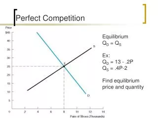
9. The Competitive Firm • Firm’s D Curve under Perfect Competition: • Horizontal demand • Cannot impact market price • E.g., Farmer Jones can double or triple Q and it has no effect on P corn. Jones is insignificant to the market exchange in Chicago, so she must accept P that a broker quotes her.

10. Industry D S supply curve A B C E Industry Price per Bushel demand curve in Chicago Firm’s demand curve S D Truckloads of Corn Total Sales in Chicago Sold by Farmer Jones in Thousands of Truckloads per Year per Year FIGURE 1. Demand Curve for a Firm under Perfect Competition $8 $8 0 1 2 3 4 0 100 200 300 400 (a) (b)

11. The Competitive Firm • Short-Run Equilibrium for the Perfectly Competitive Firm: • Profit-max Q is where MR = MC. • D (or AR curve) is horizontal. So D is the MR curve or MR = P. • If a firm ↑Q by 1 unit, it still receives the same P. • At an optimum Q: MR = P = MC → P = MC.

12. TABLE 1.Revenues, Costs, and Profits of a Competitive Firm

13. MC AC B D = MR = AR = P A FIGURE 2. Short-Run Equilibrium of the Perfectly Competitive Firm Revenue and Cost per Bushel $8 $6 4 0 50,000 Bushels of Corn per Year

14. Short-Run Profit: Graphic Representation • To measure profit graphically, compare height of D curve with height of AC curve. • Recall: Profit = TR - TC TR = P x Q TC = AC x Q • Since Q is identical, we can graphically compare P and AC to see if firm earns SR profits or losses. • If P > AC → firm earns profits or if P < AC → firm incurs losses.

15. Short-Run Profit: Graphic Representation • Profit per unit = revenue per unit (P) - cost per unit (AC). If P > AC → firm makes a profit on each unit. • E.g., AC = TC/Q = $300,000/50,000 = $6 and P = $8, so the profit per unit is $2 or vertical distance between points B and A in Fig. 2. • Total profit = profit per unit (P-AC) x Q $100,000 = $2 x 50,000 = area labeled $8 $6 A B. • MR = MC indicates profit-max Q but it doesn't show whether the firm earns profits or incurs losses. We must compare P and AC to determine this.

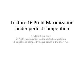
16. Short-Run Losses: Graphic Representation • If D is weak or costs are high, the firm’s most profitable option may lead to a loss. • Assume P is $4 per bushel and relevant data in Table 2. • Jones still produces Q at P = MR = MC to min. losses. • Q = 30,000 where MR  MC. • Total loss is $5,000 = per unit loss (AC - P) of $0.167 x Q of 30,000. Losses are shown by area $4 $4.16 C D in Fig. 3 below.

17. TABLE 2. Revenues, Costs, and Losses of a Competitive Firm

18. MC AC Revenue and Cost C per Bushel D D = MR = AR = P FIGURE 3. Short-Run Equilibrium of Competitive Firm with Losses $4.16 4.00 0 30,000 Bushels of Corn per Year

19. Shutdown and Break-Even Analysis • Firms can't endure a loss forever. • Sunk costs = costs that cannot be escaped in SR. • E.g., restaurant owner has signed a one-year lease on a building. • If firm shuts down → TR = 0 and TVC = 0, but TFC (or sunk costs) remain. Sometimes it is better to remain in operation until the sunk costs expire.

20. Shutdown and Break-Even Analysis • 2 rules that govern the shutdown decision: • If TR > TC → firm earns positive profits and should remain open in SR and LR. • Firm should operate in SR if TR > TVC, but should plan to close in LR if TR < TC. • Proof: • Loss if the firm stays open = TC - TR • Loss if the firm shuts down = TFC = TC - TVC • So stay open in SR if: TC - TR < TC - TVC or TR > TVC.

21. TABLE 3. The Shutdown Decision

22. Shutdown and Break-Even Analysis • In Table 3, both firms have the same TR and TFC, but differ in their TVC. • Both firms should close in LR because TC > TR. • Yet, firm A should remain open in SR because it earns $20,000 in TR above TVC, which can go toward TFC. • Firm B should close now. By operating in SR, it adds $30,000 in TVC above TR, which can be avoided by closing.

23. MC AC AVC P P 3 3 A B P P 2 2 P P 1 1 FIGURE 4. Shutdown Analysis Price 0 Quantity Supplied

24. Shutdown and Break-Even Analysis • This firm operates at a loss whether P is P1, P2, or P3. • Lowest P to keep the firm open in SR is where P  AVC. • Stay open in SR if: TR > TVC P x Q > AVC x Q Since Q is equal, P > AVC. • Firm will shut down immediately if P < AVC.

25. Shutdown and Break-Even Analysis • At P = P1→ shutdown; firm cannot cover TVC. • At P = P3→ firm earns revenues above TVC so stay open in SR and produce at pt A where P3 = MC. But, firm will close in LR as TR < TC. • At P = P2→ firm is indifferent between remaining open and closing since TR just covers TVC. If firm stays open it will produce at pt B where P2 = MC. P2 is lowest P which Q > 0 and it’s the min pt on AVC curve.

26. The Competitive Firm’s Short-run Supply Curve • SR S curve for competitive firm = portion of MC curve that lies above the min pt on AVC curve. • Supply tells us how much output is produced at different prices. • In SR: (1) If P > AVC → produce where P = MC. So for any P above pt B, MC tells us the Qs. (2) If P < AVC then Qs = 0.

27. The Competitive Industry’s Short-run Supply Curve • SR for industry: too brief a period of time for new firms to enter or old firms to leave. Number of firms is fixed. • LR for industry: long enough period of time for any firm that so chooses to enter or leave. Also, each firm can adjust its Q to fit LR costs. • SR industry S curve is horizontal summation of the individual firm's S curves. • SR industry S curve has (+) slope because individual firms have MC curves that slope upward.

28. s S E e c C s S Quantity Supplied in Quantity Supplied in Thousands of Bushels Millions of Bushels FIGURE 5. Derivation of the Industry Supply Curve Typical Corn Farmer Corn Industry $8.00 $8.00 Price per Bushel Price per Bushel 6.00 6.00 45 50 45 50 (a) (b)

29. The Competitive Industry’s Short-run Supply Curve • In Fig. 5, if 1,000 identical firms each supplied 45,000 when P = $6 → industry Qs is 45,000 x 1,000 = 45 million. Repeating this process for every P derives industry S curve. • Entry of new firms shifts SR industry S curve out. • Exit of old firms shifts SR industry S curve in.

30. The Competitive Industry • Industry S and market D determine equilibrium P and Q. • Individual firms face horizontal D curves because they are so small. If 1 firm doubled its Q, market P is unchanged. But if every firm in industry doubled their Q, ↓P to induce consumers to purchase the add. Q. • In Fig. 6, equilibrium → P = $8 and Q = 50 million. • Recall: if P = $6 → shortage = 27. ↑P toward E as frustrated buyers bid up prices.

31. S D E A C D S Quantity of Corn in Millions of Bushels FIGURE 6. Supply-Demand Equilibrium of a Competitive Industry $10.00 8.00 Price per Bushel 6.00 0 45 50 72

32. Industry and Firm Equilibrium in the Long Run • LR equilibrium may differ from SR equilibrium because: • number of firms may differ • firms can vary their plant size in LR • Thus, firm and industry cost curves differ in LR. • Firms enter or exit based on Π earned in industry. • SR profits → new firms enter • SR losses → existing firms exit • If firms earn high profits in an industry then new firms enter, forcing ↓Pas SR industry S curve shifts out.

33. MC (1,000 firms) S AC 0 D (1,600 firms) S 1 E e D 0 A a D 1 b D S 0 S 1 Quantity of Corn in Quantity of Corn in Thousands of Bushels Millions of Bushels FIGURE 7. Entry of Firms into the Competitive Industry Typical Firm Industry Price per Bushel Price per Bushel $8.00 $8.00 6.00 6.00 40 45 50 50 72 (a) (b) Typical firm earns profits at point e which encourages the entry of 600 new firms. This shifts industry S curve out and lowers P.

34. Entry of Firms into the Competitive Industry • SR profits (point e in Fig. 7) encourages 600 firms to enter which shifts industry S out and pushes P down to $6 (new SR equilibrium point A). • Existing firms react to ↓P by setting new P = MC and lowering their Q to 45,000. • At P = $6 → 1,600 firms produce 45,000 each so industry Qs = 72M. • Point A is another SR equilibrium as typical firm earns profits. Note: P > AC and per unit profits = a – b.

35. MC D AC (2,075 firms) S 2 M m D 2 S 2 D Quantity of Corn in Quantity of Corn in Thousands of Bushels Millions of Bushels FIGURE 8. LR Equilibrium of the Competitive Firm and Industry Typical Firm Industry Price per Bushel Price per Bushel $5.00 $5.00 83 40 (a) (b) Point m is a LR equilibrium where typical firm earns zero profits and produces where P = AC = MC.

36. Entry of Firms into the Competitive Industry • Entry continues until all profits are competed away. SR Industry S will shift out until P = min AC. • LR equilibrium (point m in Fig. 8) is where typical firm earns zero profits and produces where P = AC = MC. • There are no profits in LR. • SR profits → firms enter and ↓P until all profits end. • SR losses → firms leave and ↑P until all losses end.

37. Zero Economic Profit • Why do firms stay in the industry if profits are zero in LR? • Recall: economist's definition of profit includes opportunity cost of any K or L supplied by firm's owners. 0 economic Π → (+) accounting Π • E.g., if investors can earn 15% on their funds elsewhere → firm must earn 15% to cover opportunity cost of its K. If not, funds will not be given to the firm because investors will go elsewhere.

38. Zero Economic Profit • Zero economic profit indicates firms are earning the normal economy-wide rate of profit (in the accounting sense). • An industry whose K earns a higher rate of return than K invested elsewhere attracts K into the industry. This shifts SR industry S curve out and ↓P until econ Π= 0. • If K invested in an industry earns a lower return than K invested elsewhere, funds dry up in the industry. This shifts SR industry S curve in and ↑P until econ Π = 0.

39. The LR Industry Supply Curve • LR industry S curve reflects: • Entry and exit of firms → shifts SR industry S curve toward its LR position. • Each firm is freed of its sunk cost commitments → each firm is operating on its LR AC curve. • LR industry S curve = Industry’s LR AC curve because LR Π = 0, so industry P = industry LR AC. • If P > LRAC → firms enter, attracted by profits • If P < LRAC → firms exit, due to losses

40. S LRAC B S A Output in Millions of Bushels of Corn FIGURE 9. SR Industry Supply and LR Industry Average Cost If LR P = $4 and current P = $7→ firms earn $3 in economic Π on each bushel they sell → entry of new firms → S shifts out to LRAC. $7.00 Price, Average Cost per Bushel 4.00 0 70

41. Perfect Competition and Economic Efficiency • Perfect competition leads to great efficiency in LR as firms must produce where P = min LR AC curve. Thus, output of competitive industries is produced at lowest possible cost to society. • In Table 4, industry produces 12 million bushels by having 120 firms produce 100,000. • Total industry cost = AC x industry output, so total industry cost is lowest by having each firm produce at lowest AC possible.

42. TABLE 4. AC for the Firm and Total Cost for the Industry