1 / 0

Lecture 16 Profit Maximization under perfect competition

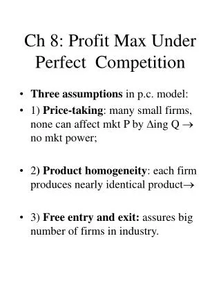
Lecture 16 Profit Maximization under perfect competition. 1. Market structure 2. Profit maximization under perfect competition 3. Supply and competitive equilibrium in the short run. Market structures.

willis
Download Presentation

Lecture 16 Profit Maximization under perfect competition

An Image/Link below is provided (as is) to download presentation Download Policy: Content on the Website is provided to you AS IS for your information and personal use and may not be sold / licensed / shared on other websites without getting consent from its author. Content is provided to you AS IS for your information and personal use only. Download presentation by click this link. While downloading, if for some reason you are not able to download a presentation, the publisher may have deleted the file from their server. During download, if you can't get a presentation, the file might be deleted by the publisher.

E N D

Presentation Transcript


  1. Lecture 16 Profit Maximization under perfect competition

    1. Market structure 2. Profit maximization under perfect competition 3. Supply and competitive equilibrium in the short run
  2. Market structures Perfect competition: many buyers and sellers, undifferentiated product, no barriers to entry or exit, perfect information Monopolistic competition – similar to perfect competition but with differentiated products (examples: clothes, computers, processed foods) Monopoly: Single seller, many buyers, barriers to entry likely (e.g., limited access to inputs, government approval) Oligopoly – Similar to monopoly but with a small number of firms. May compete (network television stations, mobile phone companies) or may collude (OPEC)
  3. Conditions for perfect competition Firms sell a standardized product Free entry and exit in long run Firms and consumers have perfect information Firms are price takers Large number of buyers and sellers Almost never perfectly satisfied but often close enough
  4. Product homogeneity The product sold by one firm is assumed to be a perfect substitute for the product sold by any other Classic examples of homogenous products: agricultural products (corn, wheat, milk, oranges, beef, sugar), gasoline, steel Often called commodities Buyers are indifferent among products from different sellers. One price in the market.
  5. Free entry and exit No significant cost that makes it difficult for new firms to enter the industry or existing firms to leave Factors of production are mobile in the long run (no entry or exit in short run by definition) Common examples of barriers to entry: Licensing requirements—bars, taxis, professions (lawyers, doctors, veterinarians), pro sports teams Access to inputs or use of technology (limited supply, patent; cost) Examples of barriers to exit: Labor contracts –can’t afford to close because costs of paying off contracts are too high In some countries, agricultural land that is unused is subject to expropriation
  6. Perfect information Firms know all the possible profit opportunities in the industry and elsewhere. Consumers know all the prices charged by firms and the product information
  7. Firms are price takers The firm has no control over the price of the products they sell. They sell at the price determined in the market. Most important condition Follows from homogeneity and free entry and exit, no firm could sell at a price other than the market price and stay in business.
  8. Large number of buyers and sellers Follows from others but is well-known and is easy to verify empirically (though there is no definition of “large”) The number of buyers and sellers is large in the sense that no individual firm can significantly affect the price of the product by changing the quantity it buys or sells.
  9. Definition of profit (π) Profit = Economic profit = total revenue minus total costs, where total cost includes implicit and explicit costs π =TR (Q) – TC (Q) Accounting profits = TR - explicit costs Accounting profit > Economic profit Difference between economic profit and accounting profit is often called “normal profit” which is the opportunity cost of owner’s resources
  10. Profit in short and long run under perfect competition π = TR(Q) – TC (Q) π = PQ – TC (Q) = PQ – (TC/Q)Q TR = PQ because firm is a price taker In short run: π = Q (P - ATC) In long run, π = Q(P - LAC)
  11. Example: Calculating total revenue, cost and profitThe following table contains firm output and cost data. (Is this short or long run?)
  12. In Class 1- Calculate Marginal Cost
  13. MC, ATC and AVC $ MC ATC AVC Q
  14. Graph of profit as a function of Q $ Q
  15. Total revenue, total cost and profit for a typical firm
  16. Marginal revenue, marginal cost and profit π = TR(Q) – TC (Q) A condition for π maximization is ∂π/∂Q = 0 ∂π/∂Q = ∂TR/∂Q - ∂TC/∂Q Marginal revenue (MR) is the change in revenue from the sale of an additional unit of Q ∂TR/∂Q When firm is a price taker, MR=P since ∂TR/∂Q =∂PQ/∂Q=P Marginal cost (MC) is the change in total cost from an additional unit of Q ∂TC/∂Q
  17. Marginal revenue, marginal cost and profit Under perfect competition, maximum profit occurs when MR=MC => P=MC ∂π/∂Q = MR - MC = 0 => MR=MC This is equivalent to marginal benefit = marginal cost
  18. Profit-Maximizing Output Level in the Short-Run
  19. Profit maximization under perfect competition Output rule in the Short‐run: If a firm is producing any output, Q should be set at the level where MC (Q) = P on the rising portion of the MC curve. Output rule in the Long‐run: If a firm is producing any output, Q should be set at the level where LMC(Q) = P on the rising portion of the LMC curve.
  20. The output rule of profit maximization If the firm is producing any output (Q), to maximize profits the firm should produce a level of output for which marginal revenue is equal to marginal cost on the rising portion of the MC curve (see thick line in graph) Output rule applies in the short and long run.
  21. Shut-down rules under perfect competition Shut‐down Rule in the Short‐run: The firm should shut down (produce nothing) if P < minimum average variable cost (min AVC). Shut‐down Rule in the Long‐run: The firm should shut down (produce nothing) if P< minimum average total cost (min LAC).
  22. Shut-down Rule in the short run: The firm should shut down (produce nothing) if P < minimum average variable cost (min AVC). P Problem here is that firm is not covering variable costs
  23. The “shut down” rule At any level of Q, if P < AVC, π < − FC π = PQ − TC = PQ − VC − FC which can be re-written as Q(P-AVC) − FC If P < AVC, then Q(P-AVC) <0 and π < -FC If Q=O, then π = − FC so firm will maximize profit by producing nothing.
  24. In class 2 – How much would the firm produce when P = 30? when P = 20? and when P = 10? $ MC ATC AVC Q
  25. Finding Q* to maximize profit using cost function A firm’s cost function (TC) = Q2- 4Q+10 and price is 20. If firm is maximizing profit, What will its output (Q) be? What will its profit be?
  26. Find Q* to maximize profit TC = Q2-4Q+10 and P = 20 Profit is maximized when MR=MC or P=MC MC= ∂TC/∂Q = 2Q-4 Set MC equal to 20 and solve for Q. 2Q-4 = 20 => Q=12
  27. If Q*=12, what is profit? TC = Q2-4Q+10 and price =20. Profit = TR-TC TR = PQ= 20*12 = 240 TC= 122-4(12)+10 = 144-48+10 = 106 Profit = TR-TC = 240-106 = 134
  28. In class 3 A firm’s cost function is TC = Q2-4Q+10 and price is 6. If firm is maximizing profit, What will its output (Q) be? What will its profit be?
  29. In the short run, the individual firm will maximize profit by producing Q where MR=MC when P is > AVC and Q=0 when P ≤ AVC
  30. In the long run, the individual firm will maximize profit by producing Q where MR=LMC when P is ≥ LAC and Q=0 when P< LAC
  31. Key differences between short and long run In the short run, a firm might still produce Q>0 even though profits are negative as long as π > -FC. If -FC> π then firm should shut down (produce Q=0). It would still have to pay fixed costs but is better off producing nothing and waiting to see if P increases A farmer can leave crops in the field if expected profit is less than fixed costs Firms can stop production and lay off wage laborers but still pay salaries In the long run, there are no fixed costs so if π <0, firm should shut down permanently.
  32. Firm supply curve in the short run (SR) Supply curve records results of firm’s profit maximization decisions In a perfectly competitive market, firm SR supply curve is the portion of the MC curve that is above AVC and the portion of Y axis (Q=0) that is below the minimum AVC.
  33. Industry and market supply functions Firm Supply (Curve/Function): the relationship between the price of a product and the quantity of the product supplied by one individual firm. Market / Industry Supply (Curve/Function): the relationship between the price of a product and the total quantity of the product supplied by all firms in the market.
  34. Market supply function is the horizontal sum of the individual firm supply functions
  35. In class 4 In the peanut butter industry, there are 100 identical firms and each has a supply function P=4+Qi. What is the industry supply function?
  36. Competitive equilibrium (market equilibrium in a perfectly competitive market)
More Related