Download
1 / 8
80 likes | 226 Views
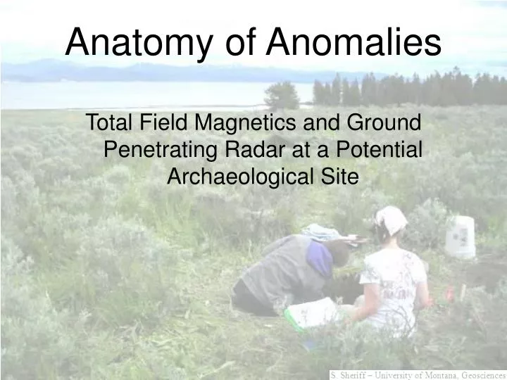
Anatomy of Anomalies. Total Field Magnetics and Ground Penetrating Radar at a Potential Archaeological Site. Raw and Decorrugated Total Magnetic Field Intensity.

E N D
Anatomy of Anomalies Total Field Magnetics and Ground Penetrating Radar at a Potential Archaeological Site
Raw and Decorrugated Total Magnetic Field Intensity The upper image shows the raw total field intensity; dots indicate acquired observations. The lower image shows diurnally corrected and decorrugated results. Horizontal dimensions are meters; the contour interval is 2 nanoteslas (nt).
Analytic Signal of the Total Magnetic Field Intensity The analytic signal (total gradient) often serves as a convenient method to help locate potential archaeological targets. Here, warm to hot colors mark larger and more likely interesting magnetic sources in the subsurface. The analytic signal, dependent on all three second order directional derivatives, is subject to noise. Distributed sources on the surface could cause any of the spots on the lower image.
Separating Deep and Shallow Equivalent Source Layers Matched bandpass filtering is an effective way to separate magnetic anomalies arising from different depths. It entails fitting the radially averaged power spectrum of the total field magnetic data with a series of power spectra corresponding to simple equivalent layers at the archaeological site. Often it is the best way to remove the effects of randomly scattered surface debris, particularly if that debris is ferromagnetic. Here, the upper image shows the field from a deep equivalent layer, the lower image is that of the shallow equivalent source; contour interval = 1 nt. Note the effective isolation of the short wavelength signal.
Overlapping (and complementary) Ground Penetrating Radar Despite rough ground conditions (fallen logs, bunchgrass, and sagebrush) we were able to acquire GPR data over part of the magnetic grid. The image shows the position of the GPR data volume collected over 10 meters of the magnetic grid. We used a 500 mhz antenna, 0.5 meter profile spacing, and trace separation of 0.05 meters while stacking 16 times per trace.
Time (or depth) Slices from the GPR Data Volume This is a time slice (horizontal section) of absolute amplitudes of the data volume averaged over 6 nanoseconds (ns) starting at 18 ns deep (just less than one meter). The black X's corroborate the highs in the analytic signal, thus these GPR features also have strong magnetic anomalies. This time slice averages over 6 ns at a depth of 21 ns (just over a meter deep). Several arcuate radar features show up in the northeast corner. There are no associated magnetic anomalies and the radar features are on the extension of the old road that cuts the grid. As shown on the next slide, these result from fluvial features. Note the dependence of the results on slight changes in depth position.
Circular GPR Features from Fluvial Structures The 6 ns GPR time slice at a depth of 21 ns (just over a meter deep). The arcuate, sub-circular features result from taking horizontal sections through the fluvial structures. The upper image shows the north (left) and east sides of the GPR volume. Everything below 0.90 meters is fluvial silts and sand as evidenced by GPR interpretation, excavation, and auguring. Those sands yield good radar reflections. The lower image highlights fluvial features which, when sliced horizontally into time slices, produce the arcuate features in the time slices .
Recommendations and Results – Total Field Magnetics and GPR • The exploration area, in open timber with deadfall, bunchgrass, and some sagebrush contains highly magnetic obsidian boulders distributed on the surface and in the shallow subsurface. The upper set of solid-dashed magenta lines shows the position of a historic road with minor excavation still visible off the map to the east (right). The lower magenta lines outline a near-rectilinear anomaly with high gradient edges. The numbered anomalies indicate recommended positions for test units based on the combined magnetic and GPR results. The results of test units: • Position 1 yielded cultural artifacts • Positions 2, 3, and 4 yielded only boulders. Although each individual anomaly has the character of a boulder with remanent magnetization their concentration and alignment was promising • Position 5 has a fire hearth at about 0.8 meters • Position 6 has a rock concentration dated at 3,090 years.