Download
1 / 67
710 likes | 1.05k Views
Reconstruction of Solid Models from Oriented Point Sets. Misha Kazhdan Johns Hopkins University. Shape Spectrum. There are many ways to represent a shape: Point Set Polygon Soup Polygonal Mesh Solid Model. Equivalence of Representations. There are many ways to represent a shape:

E N D
Reconstruction of Solid Models from Oriented Point Sets Misha Kazhdan Johns Hopkins University
Shape Spectrum There are many ways to represent a shape: • Point Set • Polygon Soup • Polygonal Mesh • Solid Model
Equivalence of Representations There are many ways to represent a shape: • Point Set • Polygon Soup • Polygonal Mesh • Solid Model In one direction, the transition between representations is straight-forward
Equivalence of Representations There are many ways to represent a shape: • Point Set • Polygon Soup • Polygonal Mesh • Solid Model ? In one direction, the transition between representations is straight-forward The challenge is to transition in the other direction
Equivalence of Representations There are many ways to represent a shape: • Point Set • Polygon Soup • Polygonal Mesh • Solid Model The goal of this work is to define a method for computing solid models from oriented point sets.
Applications • Surface Blending Disjoint Model “Zippered” Model
Applications • Surface Blending • Hole-Filling Model with Hole Water-Tight Model
Applications • Surface Blending • Hole-Filling • Compression Geometry + Topology Representation Geometry Representation
Applications • Surface Blending • Hole-Filling • Compression • Simplification Original Model871,000 Triangles Simplified Model95,000 Triangles
Related Work Three general approaches: • Computational Geometry Boissonnat, 1984 Edelsbrunner, 1984 Amenta et al., 1998 Dey et al., 2003 • Surface Fitting Terzopoulos et al., 1991 Chen et al., 1995 • Implicit Function Fitting Hoppe et al., 1992 Curless et al., 1996 Whitaker, 1998 Carr et al., 2001 Davis et al., 2002 Ohtake et al., 2004 Turk et al., 2004 Shen et al., 2004
Related Work • Implicit Function Fitting • Use the point samples to define an function whose values at the sample positions are zero. <0 0 >0 Sample Points F(x,y)
Related Work • Implicit Function Fitting • Use the point samples to define an function whose values at the sample positions are zero. • Extract the iso-surface with iso-value equal to zero. <0 F(x,y) =0 0 F(x,y)>0 F(x,y)<0 >0 Sample Points F(x,y)=0
Related Work • Implicit Function Fitting • Use the point samples to define an function whose values at the sample positions are zero. • Extract the iso-surface with iso-value equal to zero. >0 F(x,y) =0 0 F(x,y)<0 F(x,y)>0 How should we define the implicit function so that the reconstruction fits the samples? <0 Sample Points F(x,y)=0
Outline • Introduction • Related Work • Approach • The Divergence Theorem • Reduction to Volume Integration • Implementation • Results • Conclusion
Divergence Theorem Given a vector field F and a region V: The volume integral of F over V and the surface integral of F over V are equal: = V V
Reduction to Volume Integration (Step 1) Characteristic Function: The characteristic functionVof a solid V is the function: V
Reduction to Volume Integration (Step 2) Fourier Coefficients: The Fourier coefficients of the characteristic function give an expression of Vas a sum of complex exponentials:
Reduction to Volume Integration (Step 3) Volume Integration: The Fourier coefficients of the characteristic function V can be obtained by integrating:
Reduction to Volume Integration (Step 3) Volume Integration: The Fourier coefficients of the characteristic function V can be obtained by integrating: since the characteristic function is one inside of V and zero everywhere else.
Applying the Divergence Theorem Surface Integration If Flmn(x,y,z) is any function whose divergence is equal to the (l,m,n)-th complex exponential:applying the Divergence Theorem, the volume integral can be expressed as a surface integral:
Reconstruction Algorithm Given an oriented point sample {(pi,ni)}: • Compute a Monte-Carlo approximation of the Fourier coefficients of the characteristic function: • Apply the inverse Fourier Transform to obtain the characteristic function. • Extract the reconstruction an iso-surface of the characteristic function
Algorithm Implementation • Efficiency: We show that the computation of the Fourier coefficients is actually a convolution, reducing the reconstruction complexity: O(R5) → O(R3logR). • Non-Uniformity: We provide a simple heuristic for assigning weights to samples that may be non-uniformly distributed.
Outline • Introduction • Related Work • Approach • Results • Resolution • Sample Count • Non-Uniformity • Related Work • Conclusion
Results (Resolution) 100,000 Points 100,000 Points 100,000 Points res=643 tris=11,672 time<0:01 res=1283 tris=49,008 time=0:01 res=2563 tris=199,796 time=0:07
Results (Sample Count) 1000 Points 10,000 Points 100,000 Points res=2563 tris=200,704 time=0:07 res=2563 tris=199,796 time=0:07 res=2563 tris=206,216 time=0:07
Results (Non-Uniform Sampling) 100,000 Points 100,000 Points 100,000 Points res=2563 tris=199,712 time=0:09 res=2563 tris=111,680 time=0:09 res=2563 tris=220,324 time=0:09
Results(Non-Uniform Sampling / Related Work) 100,000 Points 100,000 Points 100,000 Points RBF Reconstruction† MPU Reconstruction‡ Our Reconstruction res=2563 tris=302,000 time=5:23 res=2563 tris=288,000 time=0:39 res=2563 tris=286,916 time=0:09 ‡Ohtake et al. ACM TOG ‘03 †Carr et al. SIGGRAPH ‘01
Results (Noise / Related Work) Original RBF Reconstruction† Our Reconstruction MPU Reconstruction‡ res=2563 tris=200,000 time=24:10 points=100,000 res=2563 tris=205,000 time=2:14 points=100,000 res=2563 tris=174,824 time=0:07 points=100,000 ‡Ohtake et al. ACM TOG ‘03 †Carr et al. SIGGRAPH ‘01
Outline • Introduction • Related Work • Approach • Results • Conclusion
Conclusion Properties: • Fast and simple to compute • Independent of topology • Robust to non-uniform sampling • Robust to noise • O(R3) memory footprint for O(R2) reconstruction
Conclusion Theoretical Contribution: • Transformed the surface reconstruction problem into a Volume integral • Used the Divergence Theorem to express the integral as a surface integral • Used Monte-Carlo integration to approximate the surface integral as a summation over an oriented point sample
Conclusion We presented an algorithm for reconstruction that proceeds in three simple steps:
Conclusion We presented an algorithm for reconstruction that proceeds in three simple steps: • Splat the oriented points into a voxel grid
Conclusion We presented an algorithm for reconstruction that proceeds in three simple steps: • Splat the oriented points into a voxel grid • Convolve with a fixed filter
Conclusion We presented an algorithm for reconstruction that proceeds in three simple steps: • Splat the oriented points into a voxel grid • Convolve with a fixed filter • Extract the iso-surface
Thank You Source and Executables: http://www.cs.jhu.edu/~misha/Reconstruct3D
Choosing the Functions Flmn There are many solutions to the equation:
Choosing the Functions Fl,m,n There are many solutions to the equation: Examples:
Choosing the Functions Fl,m,n There are many solutions to the equation: Examples:
Choosing the Functions Fl,m,n There are many solutions to the equation: In our implementation, we choose the function: This is the unique definition of Flmn with the property that the reconstruction commutes with translation and rotation.
Choosing the Functions Fl,m,n 30o 45o 0o Does not Commute: Commutes:
Choosing the Functions Fl,m,n Does not Commute: Commutes:
Non-Uniform Samples Challenge: In a direct implementation of Monte-Carlo integration, it is assumed that the samples are uniformly distributed:
Non-Uniform Samples Challenge: In a direct implementation of Monte-Carlo integration, it is assumed that the samples are uniformly distributed: However, often the oriented point samples may not be uniformly distributed over the surface: • Parts of scans may overlap • Faces parallel to the view plane may be more densely sampled • Compressed representations may store fewer points in regions of low curvature
Non-Uniform Samples Challenge: If we have a sampling density i associated to each sample xi, we can modify the summation:
Non-Uniform Samples Challenge: If we have a sampling density i associated to each sample xi, we can modify the summation: However, when we get an oriented point sample, we usually aren’t given the sampling density at each sample.
Non-Uniform Samples Challenge: If we have a sampling density i associated to each sample xi, we can modify the summation: However, when we get an oriented point sample, we usually aren’t given the sampling density at each sample. Non-Uniform Samples Unweighted Reconstruction
Non-Uniform Samples Approach: Compute the sampling density at each sample by counting the number of samples around it: