Download
1 / 44
450 likes | 715 Views
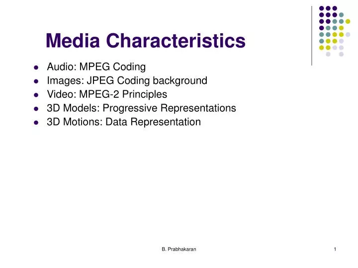
Media Characteristics. Audio: MPEG Coding Images: JPEG Coding background Video: MPEG-2 Principles 3D Models: Progressive Representations 3D Motions: Data Representation. MPEG Audio Features. MPEG Audio Layers Layer 1 allows for a maximal bit rate of 448 Kbits/second.

E N D
Media Characteristics • Audio: MPEG Coding • Images: JPEG Coding background • Video: MPEG-2 Principles • 3D Models: Progressive Representations • 3D Motions: Data Representation B. Prabhakaran
MPEG Audio Features • MPEG Audio Layers • Layer 1 allows for a maximal bit rate of 448 Kbits/second. • Layer 2 allows for 384 Kbits/second • Layer 3 for 320 Kbits/second. • All samplings at 16 bits. • Sampling frequencies: CD (compact disc) digital audio (44.1 kHz) and digital audio tapes (48 kHz); Sampling at 32 kHz is also available. B. Prabhakaran
MPEG Audio Coding B. Prabhakaran
MPEG Audio Coding… • Uncompressed audio transformed into 32 non-interleaved sub-bands using Fast Fourier Transform (FFT). • Amplitude and noise level of signal in each sub-band determined using a psycho-acoustic model. • Next, quantization of the transformed signals. • MPEG audio layers 1 and 2 are PCM-encoded. Layer 3: Huffman coded. • Types of channels • Single channel, two independent channels, or one stereo channel. • Stereo channels: processed independently or jointly. Joint stereo exploits redundancy of both channels B. Prabhakaran
MPEG-2 Audio • Different channels: • 5 full bandwidth channels (left, right, center, and two surround channels). • Additional low frequency enhancement (LFE) channel. • Up to seven commentary or multilingual channel. • Sampling rates defined for MPEG-2 audio include 16 KHz, 22.05KHz, and 24 KHz B. Prabhakaran
JPEG Compression • Modes of compression • Lossy Sequential DCT-based Mode: also known as baseline process; Needs to be supported by every JPEG implementation. • Expanded Lossy DCT-based Mode: Provides an additional set of further enhancements to the baseline mode. • Lossless Mode: Allows perfect reconstruction of the original image; lower compression ratio. • Hierarchical Mode: consists of images with different resolutions generated using the methods described above. B. Prabhakaran
Image Preparation • Source image can have up to 255 components (instead of only three components Y,U, and V). • E.g., components of an image can be the color components (Red R, Green G, Blue B) or luminance components (Luminance Y, chrominance U and V). • Each component of the image may have the same or different resolution, in terms of the number of pixels in the horizontal and vertical axis. B. Prabhakaran
Image Preparation .. • In JPEG, gray scale image will consist of a single component. • RGB image in JPEG has three components with resolutions: • Y1 = Y2 = Y3 and X1 = 2X2 = 2X3. B. Prabhakaran
Image Preparation … • Each pixel represented by p bits; values 0 - 2p-1. • Value of p depends on the mode of compression. • Lossy modes use either 8 or 12 bits per pixel. • Lossless modes use 2 upto 12 bits per pixel. • All pixels of all components within the same image are coded with the same number of bits. • An application can have different number of bits per pixel, provided a suitable transformation of the image to the well defined numbers of bits in the JPEG standard. B. Prabhakaran
Non-Interleaved Ordering • Data processed in one component completely before processing the next component. • Within a component: processing from left-to-right and then top-to-bottom. • While decoding components: display one after the other. E.g., in RGB-encoded image, red component will be presented first, green component next, and then the blue component. B. Prabhakaran
Interleaving of Components • JPEG divides each component of the image to be compressed into equal number of regions. • Then, specify a Minimum Coded Unit (MCU). • MCU comprises of exactly one region in each component. B. Prabhakaran
Interleaving of Components .. • MCU1 consists of regions R1 in components C1 and C2. • Data units within one region are ordered as in the earlier way: left-to-right and top-to-bottom. • MCU1 in Example figure: • C100 C101 C110 C111 C200 C201; • MCU2: • C102 C103 C112 C113 C202 C203 and so on. B. Prabhakaran
Lossy Sequential Mode • Uncompressed image: divided into blocks of 8 X 8 pixels. • Order of blocks: determined by the MCU. These blocks are passed to the image processing phase. B. Prabhakaran
Lossy Sequential Mode • Values of each pixel is shifted in the range -128 to 127, with zero as the center. Achieved by Discrete Cosine Transformation (DCT). • For a block of 8 X 8 pixels, shifted values are represented by Sxy, 0 ≤ x ≤ 7, 0 ≤ y ≤ 7. • Each of these values are transformed using Forward DCT (FDCT). • Above FDCT transformation has to be done 64 times per block, resulting in 64 coefficients Suv per block. • Cosine expressions depend on x, y, u, and v, but not on Sxy. Computation can be optimized to take advantage of this fact. B. Prabhakaran
Lossy Sequential Mode .. • FDCT maps the value from the time to the frequency domain. • Each coefficient of Suv can be regarded as a two-dimensional frequency. • Coefficient S00, the DC-coefficient, corresponds to the lowest frequency in • both dimensions. Also describes the fundamental color of the 8 X 8 pixels • block. • Rest of the coefficients known as AC-coefficients. B. Prabhakaran
Quantization Phase • FDCT coefficients in a block may have low or zero values, if the block has only one predominant color. • Entropy encoding is used for further compression • Each of the 64 coefficient value is scaled by a factor Q, the quantization factor. • E.g., the quantized value of the DC-coefficient, SQ00, is : SQ00 = S00 / Q. • In most cases, quantization is not done in a uniform manner. • Low frequencies of the FDCT coefficients describe the boundaries among regions in the image being compressed. • If low frequency coefficients are quantized in a very coarse manner (i.e., with high values of Q), boundaries in the reconstructed image may not be as sharp. B. Prabhakaran
Quantization Phase • Low frequency coefficients quantized in finer manner (i.e., with lower values of Q) than higher frequency ones. • Table with 64 entries used for representing the values of the quantization factor Q, for each of the 64 FDCT coefficients. • Quantization of each coefficient is: SQuv = Suv / Quv, Quv the quantization factor for uvth coefficient. B. Prabhakaran
Quantization Phase.. B. Prabhakaran
Entropy Encoding • DC-coefficients encoded as difference of the current DC-coefficient and the previous one: for block i, difference in DC-coefficients is DCi - DCi-1. • Further processing done only on these differences. • AC-coefficients are processed in the zig-zag order shown earlier. • zig-zag sequence describes an increasing order of the frequencies of the AC-coefficients. B. Prabhakaran
Entropy Encoding • Lower frequency AC-coefficients have higher values than higher frequencies ones (which are usually very small or zero). • Hence, zig-zag ordering of AC-coefficients produces a sequence where similar values will be together. • Such a sequence is highly suitable for efficient entropy encoding. • Next step: run-length encoding of zero values. JPEG specifies Huffman and Arithmetic encoding. (Arithmetic encoding is protected by a patent). • For the lossy JPEG mode (i.e., the baseline process), only Huffman encoding is allowed to be used. B. Prabhakaran
Image Reconstruction • Decompress the data in Huffman/Arithmetic coded form. • Dequantization is then performed: Ruv = SQuv X Quv. Must use the same table as the one used in the quantization process. • Dequantized DCT coefficients are then subject to IDCT (Inverse DCT). • If FDCT and IDCT can determine the values with full precision, reconstruction can be lossless (assuming lossless quantization). • However, precision is restricted and hence the reconstruction process is lossy. B. Prabhakaran
Image Reconstruction B. Prabhakaran
Expanded Lossy Mode • Progressive representation realized by expansion of quantization. • Expansion done by addition of an output buffer to the quantizer, storing all coefficients of the quantized DCT. • Encoding process follows either: • Encoder processes DCT-coefficients of low frequencies successively (low frequencies describe border outlines). Hence, encoding low frequency coefficients successively decode the boundaries of various objects successively. • Another approach: use all the DCT-coefficients in the encoding process but single bits are differentiated according to their significance (i.e., most significant bit first and then the least significant bits are encoded). B. Prabhakaran
Progressive Spectral Selection • DCT coefficients are grouped into several spectral bands. • Low-frequency DCT coefficients sent first, and then higher-frequency coefficients. E.g., • Band 1: DC coefficients only • Band 2: AC1 and AC2 coefficients • Band 3: AC3, AC4, AC5, and AC6 coefficients • Band 4: AC7 … AC63 coefficients Bits n-1 band2 band3 band4 band1 AC3 - AC6 AC7 … AC63 AC1 & AC2 DC 0 B. Prabhakaran
Prog. Successive Approximation • All DCT coefficients sent first with lower precision. • Then refined in later scans. E.g., • Band 1: All DCT coefficients divided by 4. • Band 2: All DCT coefficients divided by 2 • Band 3: All DCT coefficients at full resolution Bits n-1 band1 band2 band3 0 DC AC1 AC2 AC63 B. Prabhakaran
Combined Progressive … • Combines both spectral & successive approximations • SCAN 1: DC band 1; Scan 2: AC band 1 • Scan 3: AC b2; Scan 4: AC b3; Scan 5: AC b4; • Scan 6: AC b5; Scan 7: DC b2; Scan 8: AC b6 Bits n-1 DC b1 AC b2 AC b3 AC b1 AC b5 AC b4 DC b2 AC b6 0 DC AC1 AC2 AC63 B. Prabhakaran
Lossless Mode • This mode work on single pixel of an image (instead of 8 X 8 pixels block). So, no processing to be done as part of the image preparation phase. • Each pixel can be encoded with 2 to 8 bits. Image preparation and quantization phases use a predictive technique (instead of a transformation oriented DCT technique). B. Prabhakaran
Lossless Mode.. • 8 possible predictor values are defined for each pixel based on the values of the adjacent pixels. • Table describes predictors for pixel X • 0 No Prediction 1 X = A • 2 X = B 3 X = C • 4 X = A + B - C 5 X = A + (B - C) / 2 • 6 X = B + (A - C) / 2 7 X = (A + B)/2 • For each pixel, the number of the chosen predictors as well as the difference of the prediction to the actual value are entropy encoded. X B. Prabhakaran
Hierarchical JPEG • Progressive JPEG at multiple resolutions R n Image Res 2 Image Res 1 B. Prabhakaran
Video Compression • Asymmetric Applications • Compression process is performed only once and at the time of storage. E.g., on-Demand servers (such as Video-on-Demand and News-on-Demand) and electronic publishing (travel guides, shopping guides, and educational materials). • Symmetric Applications • Equal use of compression and decompression process. • E.g., information generated through video cameras or by editing pre-recorded material. • Video conferencing, video telephone applications involve generation, compression, and decompression of information generated through video cameras. • Desktop video publishing applications require edit operations on pre-recorded material. B. Prabhakaran
Desirable Features for Video Compression • Random Access • Fast Forward / Rewind • Reverse Playback • Audio-Visual Synchronization • Robustness to Errors • Coding / Decoding Delay • Edit ability • Format Flexibility • Cost Tradeoffs B. Prabhakaran
MPEG Standard • MPEG-Video: compression of video signals at about 1.5 Mbits per second. • MPEG-Audio: compression of digital audio signal at the rates of 64, 128, and 192 kbps per channel. • MPEG-System deals with the issues relating to audio-visual synchronization. • Also handles multiplexing of multiple compressed audio and video bit streams. B. Prabhakaran
MPEG Video • Primary aim of MPEG-Video is to compress a video signal to a bit rate of about 1.5 Mbits/s with an acceptable quality. • MPEG is often termed a generic standard, implying that it is independent of a particular application. • Benefited from other following standards. : • JPEG • H.261: standard was already availableduring MPEG standardization. MPEG technique is more advanced than H.261. B. Prabhakaran
MPEG Video • Two nearly conflicting requirements. • Random access requirements for MPEG video are best satisfied with pure intra-frame coding. • High compression rates are not possible unless a fair amount of inter-frame coding is done. • Intra-frame coding: targets spatial redundancy reduction. • Inter-frame coding: targets temporal redundancy reduction. • Delicate balance between inter- and intra-frame coding. B. Prabhakaran
Temporal Redundancy Reduction • Temporal redundancies present in video when subsequent frames carry similar but slightly varying content. • E.g., video frames of a person walking in a street show a gradual variation in the contents based on the walking speed of the person. • Most widely used techniques for achieving temporal redundancy reduction is motion compensation. • Motion information comprises of the amplitude and the direction of displacement of the contents. • MPEG uses block-based motion compensation technique. B. Prabhakaran
Temporal Redundancy Reduction • Significant cost associated with motion information coding. • Hence, 16 X 16 bit blocks are chosen as motion compensation units (MCUs), called macro-blocks. • Two types of motion compensation are applied over these macro-blocks. • Causal predictors (Predictive coding): i.e., generate the contents of a subsequent frame based on the motion information and the contents of the current one. • Non-causal predictors (interpolative coding): Frame coded based on both a previous and a successive frame. B. Prabhakaran
Interpolative Coding • E.g, frame 10 coded based on both frames 5 and 14. • Interpolated frames also termed bidirectional frames (B-frames). • Signal to be reconstructed for block x in frame i obtained by adding a correction term to a combination of blocks in frames i-1 and i+1. B. Prabhakaran
Interpolative Coding • Advantages of interpolative coding: • Compression obtained using interpolative coding is very high. • Results in better noise reduction: the coded block is based on both a past and a future frame. • Helps in efficiently coding new blocks (i.e., the blocks that are not present in the future) in the frame to be coded. New blocks may be properly predicted from the future frame. B. Prabhakaran
Predictive Coding • E.g, frame 10 coded based on ONLY frame 5. B. Prabhakaran
MPEG Frame Sequence B. Prabhakaran
Motion Estimation Previous Frame Current Frame Future Frame • Interpolation for motion estimation: B = (A + C) / 2. A B C B. Prabhakaran
Motion Estimation … • MPEG does not specify the motion estimation technique. • Block-matching techniques likely to be used. Goal: • Estimation motion of a n X m block in the present frame with respect to a previous or a future frame. • Block is compared to with a corresponding block within a search area G of size (m + 2p X n + 2p) in the previous/future frame. • Typical: n = m = 16 (16 X 16 pixels) and parameter p = 6. n m p p Search Area G B. Prabhakaran
Block Matching Approaches • Exhaustive Search or brute force • 3-step search • 2-D Logarithmic search • Conjugate direction search • Parallel hierarchical 1-D search • Modified pixel-difference classification B. Prabhakaran
MPEG Layers • Context unit • Random access unit • Primary coding unit • Resynchronization unit • Motion compensation • DCT unit • Sequence Layer • Group of Pictures • Picture Layer • Slice Layer • Macro-blocks • Blocks B. Prabhakaran