Download
1 / 14
290 likes | 2.6k Views
Sect. 2.5: Advantages of a Variational Principle Formulation. HP δ∫ L dt = 0 (limits t 1 < t < t 2 ). An example of a variational principle . Most useful when a coordinate system-independent Lagrangian L = T - V can be set up.

E N D
Sect. 2.5: Advantages of a Variational Principle Formulation • HP δ∫Ldt = 0 (limits t1 < t < t2). An example of a variational principle. • Most useful when a coordinate system-independent Lagrangian L = T - V can be set up. • HP: “Elegant”. Contains all of mechanics of holonomic systems in which forces are derivable from potentials. • HP: Involves only physical quantities (T, V) which can be generally defined without reference to a specific set of generalized coords. A formulation of mechanics which is independent of the choice of coordinate system!
HP δ∫Ldt = 0(limits t1 < t < t2). • From this, we can see (again) that the Lagrangian Lis arbitrary to within the derivative(dF/dt) of an arbitrary functionF = F(q,t). • If we form L´ = L + (dF/dt) & do the integral, ∫L´dt, we get ∫Ldt + F(q,t2) - F(q,t1). By the definition of δ, the variation at t1 & t2 is zero δ∫L´dt will not depend on the end points. • Another advantage to HP: Can extend Lagrangian formalism to systems outside of classical dynamics: • Elastic continuum field theory • Electromagnetic field theory • QM theory of elementary particles • Circuit theory!
Lagrange Applied to Circuit Theory • System: LR Circuit (Fig.) Battery, voltage V, in series with inductor L & resistor R (which will give dissipation). Dynamical variable = charge q. PE = V = qV KE = T = (½)L(q)2 Lagrangian: L = T - V Dissipation Function: (last chapter!) ₣= (½)R(q)2 = (½)R(I)2 Lagrange’s Eqtn (with dissipation): (d/dt)[(L/q)] - (L/q) + (₣/q) = 0 switch
Lagrange Applied to RL circuit • Lagrange’s Eqtn (with dissipation): (d/dt)[(L/q)] - (L/q) + (₣/q) = 0 V = Lq + Rq I = q = (dq/dt) V = LI + RI Solution, for switch closed at t = 0 is: I = (V/R)[1 - e(-Rt/L)] Steady state (t ): I = I0 = (V/R)
Mechanical Analogue to RL circuit • Mechanical analogue: Sphere, radius a, (effective) mass m´, falling in a const density viscous fluid, viscosity η under gravity. m´ m - mf , m actual mass, mf mass of displaced fluid (buoyant force acting upward: Archimedes’ principle) • V = m´gy, T = (½)m´v2, L = T - V (v = y) Dissipation Function: ₣= 3πηav2 Comes from Stokes’ Law of frictional drag force: Ff = 6πηav and (Ch. 1 result that) Ff = - v₣ Lagrange’s Eqtn (with dissipation): (d/dt)[(L/y)] - (L/y) + (₣/y) = 0
V = m´gy, T = (½)m´v2, L = T - V (v = y) Dissipation Function: ₣= 3πηav2 Comes from Stokes’ Law frictional drag force: Ff = 6πηav and (Ch. 1 result that) Ff = - v₣ Lagrange’s Eqtn (with dissipation): (d/dt)[(L/y)] - (L/y) + (₣/y) = 0 m´g = m´y + 6πηay Solution, for v = y starting from rest at t = 0: v = v0 [1 - e(-t/τ)]. τ m´ (6πηa)-1Time it takes sphere to reach e-1 of its terminal speedv0. Steady state (t ):v = v0 = (m´g)(6πηa)-1 = gτ = terminal speed.
Lagrange Applied to Circuit Theory • System: LC Circuit (Fig.) Inductor L & capacitor C in series. Dynamical variable = charge q. Capacitor acts a PE source: PE = (½)q2C-1, KE = T = (½)L(q)2 Lagrangian: L = T - V (No dissipation!) Lagrange’s Eqtn: (d/dt)[(L/q)] - (L/q) = 0 Lq + qC-1 = 0 Solution (for q = q0at t = 0): q = q0 cos(ω0t), ω0= (LC)-(½) ω0natural or resonant frequency of circuit
Mechanical Analogue to LC Circuit • Mechanical analogue: Simple harmonic oscillator (no damping) mass m, spring constant k. • V = (½)kx2, T = (½)mv2, L = T - V (v = x) Lagrange’s Eqtn: (d/dt)[(L/x)] - (L/x) = 0 mx + kx = 0 Solution (for x = x0at t = 0): x = x0 cos(ω0t), ω0 = (k/m)½ ω0 natural or resonant frequency of circuit
Circuit theory examples give analogies: Inductance L plays an analogous role in electrical circuits that massm plays in mechanical systems (an inertial term). ResistanceRplays an analogous role in electrical circuits that viscosityηplays in mechanical systems (a frictional or drag term). CapacitanceC (actually C-1) plays an analogous role in electrical circuits that a Hooke’s “Law” type spring constantk plays in mechanical systems (a “stiffness” or tensile strength term).
With these analogies, consider the system of coupled electrical circuits (fig): Mjk = mutual inductances! • Immediately, can write Lagrangian: L = (½)∑jLj(qj)2 + (½)∑j,k(j)Mjkqjqk - (½) ∑j(1/Cj)(qj)2 + ∑jEj(t)qj Dissipation function:₣ = (½)∑jRj(qj)2
Lagrangian: L = (½)∑jLj(qj)2 + (½)∑j,k(j)Mjkqjqk - (½)∑j(1/Cj)(qj)2 + ∑jEj(t)qj Dissipation function:₣ = (½)∑jRj(qj)2Lagrange’s Eqtns: (d/dt)[(L/qj)] - (L/qj) + (₣/qj) = 0 Eqtns of motion (the same as coupled, driven, damped harmonic oscillators!) Lj(d2qj/dt2) + ∑k(j)Mjk(d2qk/dt2) + Rj(dqj/dt) +(1/Cj)qj = Ej(t)
Describe 2 different physical systems by Lagrangians of the same mathematical form (circuits & harmonic oscillators): ALL results & techniques devised for studying & solving one system can be taken over directly & used to study & solve the other. Sophisticated studies of electrical circuits & techniques for solving them have been very well developed. All such techniques can be taken over directly & used to study analogous mechanical (oscillator) systems. These have wide applicability to acoustical systems. Also true in reverse.
HP & resulting Lagrange formalism can be generalized to apply to subfields of physics outside mechanics. • Similar variational principles exist in other subfields: Yielding Maxwell’s Eqtns (E&M) the Schrödinger Eqtn Quantum Electrodynamics Quantum Chromodynamics, …..etc.