Download
1 / 56
570 likes | 849 Views
A variational formulation for higher order macroscopic traffic flow models of the GSOM family. J.P. Lebacque UPE-IFSTTAR-GRETTIA Le Descartes 2, 2 rue de la Butte Verte F93166 Noisy-le-Grand, France Jean-patrick.lebacque@ifsttar.fr M.M. Khoshyaran E.T.C. Economics Traffic Clinic

E N D
A variational formulation for higher order macroscopic trafficflow models of the GSOM family J.P. Lebacque UPE-IFSTTAR-GRETTIA Le Descartes 2, 2 rue de la Butte Verte F93166 Noisy-le-Grand, France Jean-patrick.lebacque@ifsttar.fr M.M. Khoshyaran E.T.C. Economics Traffic Clinic 34 Avenue des Champs-Elysées, 75008, Paris, France www.econtrac.com ISTTT 20, July 17-19, 2013
Outline of the presentation • Basics • GSOM models • Lagrangian Hamilton-Jacobi and variational interpretation of GSOM models • Analysis, analytic solutions • Numerical solution schemes ISTTT 20, July 17-19, 2013
Scope • The GSOM model is close to the LWR model • It isnearly as simple (non trivial explicit solutions fi) • But itaccounts for driver variability (attributes) • More scope for lagrangianmodeling, driver interaction, individualproperties • Admits a variational formulation • Expectedbenefits: numericalschemes, data assimilation ISTTT 20, July 17-19, 2013
The LWR model ISTTT 20, July 17-19, 2013
The LWR model in a nutshell (notations) • Introduced by Lighthill, Whitham (1955), Richards (1956) • The equations: • Or: ISTTT 20, July 17-19, 2013
Solution of the inhomogeneous Riemann problem • Analytical solutions, boundary conditions, nodemodeling Density Position ISTTT 20, July 17-19, 2013
Demand Supply The LWR model: supply / demand • the equilibrium supply and demand functions (Lebacque, 1993-1996) ISTTT 20, July 17-19, 2013
The LWR model: the min formula • The local supply and demand: • The min formula • Usage: numerical schemes, boundary conditions →intersection modeling ISTTT 20, July 17-19, 2013
Inhomogeneous Riemann problem (discontinuous FD) • Solution with Min formula • Can berecovered by the variational formulation of LWR (Imbert MonneauZidani 2013) Time (a,0 ) (b,0 ) (a ) (b ) Position ISTTT 20, July 17-19, 2013
GSOM models ISTTT 20, July 17-19, 2013
GSOM (Generic second ordermodelling) models • (Lebacque, Mammar, Haj-Salem 2005-2007) • In a nutshell • Kinematicwaves = LWR • Driver attributedynamics • Includesmanycurrentmacroscopicmodels ISTTT 20, July 17-19, 2013
GSOM Family: description • Conservation of vehicles(density) • Variable fundamental diagram, dependent on a driver attribute (possibly a vecteur) I • Equation of evolution for Ifollowing vehicle trajectories (example: relaxation) ISTTT 20, July 17-19, 2013
GSOM: basic equations Conservation des véhicules Dynamics of I along trajectories Variable fundamental Diagram ISTTT 20, July 17-19, 2013
Example 0: LWR (Lighthill, Whitham, Richards 1955, 1956) • No driver attribute • One conservation equation ISTTT 20, July 17-19, 2013
Example 1: ARZ (Aw,Rascle 2000, Zhang,2002) • Lagrangien attribute I= difference between actual and mean equilibrium speed ISTTT 20, July 17-19, 2013
Increasing values of I Example 2: 1-phase Colombo model (Colombo 2002, Lebacque MammarHaj-Salem 2007) • Variable FD (in the congested domain + critical density) • The attribute Iis the parameter of the family of FDs ISTTT 20, July 17-19, 2013
Fundamental Diagram (speed-density) ISTTT 20, July 17-19, 2013
modéle 2-phase modéle 1-phase Example 2 continued (1-phase Colombo model) • 1-phase vs 2-phase: Flow-density FD ISTTT 20, July 17-19, 2013
Example 3: Cremer-Papageorgiou • Based on the Cremer-Papageorgiou FD (Haj-Salem 2007) ISTTT 20, July 17-19, 2013
Example 4: « multi-commodity » models • GSOM Model • + advection (destinations, vehicle type) • = multi-commodity GSOM ISTTT 20, July 17-19, 2013
Example 5: multi-lane model • Impact of multi-lanetraffic • Two states: congestion (stronglycorrelatedlanes) et fluid (weaklycorrelatedlanes) • 2 FDsseparated by the phase boundaryR(v) • Relaxation towardseachregime • eulerian source terms ISTTT 20, July 17-19, 2013
Example 6: Stochastic GSOM (Khoshyaran Lebacque 2007-2008) • Idea: • Conservationof véhicles • Fundamental Diagram depends on driver attributeI • Iis submitted to stochastic perturbations (other vehicles, traffic conditions, environment) ISTTT 20, July 17-19, 2013
Two fundamental properties of the GSOM family (homogeneous piecewise constant case) • 1.discontinuities of Ipropagate with the speed v of traffic flow • 2.If the invariant Iis initially piecewise constant, it stays so for all times t > 0 • ⇒On any domain on which I is uniform the GSOM model simplifies to a translated LWR model (piecewise LWR) ISTTT 20, July 17-19, 2013
rr vr rl vl x FDl FDr Inhomogeneous Riemann problem • I = Il in all of sector (S) • I = Ir in all of sector (T) ISTTT 20, July 17-19, 2013
Generalized (translated) supply- Demand (Lebacque MammarHaj-Salem 2005-2007)Example: ARZ model • TranslatedSupply / Demand = supplyrespdemand for the « translated » FD (withresp to I ) ISTTT 20, July 17-19, 2013
Example of translatedsupply / demand: the ARZ family ISTTT 20, July 17-19, 2013
Solution of the Riemann problem (summary) • Define the upstream demand, the downstream supply (which depend on Il ): • The intermediate stateUm is given by • The upstream demand and the downstream supply (as functions of initial conditions) : • Min Formula: ISTTT 20, July 17-19, 2013
Applications • Analytical solutions • Boundary conditions • Intersection modeling • Numericalschemes ISTTT 20, July 17-19, 2013
Lagrangian GSOM; HJ and variationalinterpretation ISTTT 20, July 17-19, 2013
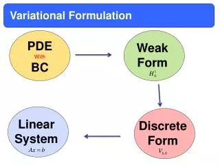
Variational formulation of GSOM models • Motivation • Numericalschemes (grid-free cfMazaré et al 2011) • Data assimilation (floatingvehicle / mobile data cf Claudel Bayen 2010) • Advantages of variationalprinciples • Difficulty • Theorycomplete for LWR (Newell, Daganzo, also Leclercq Laval for variousrepresentations ) • Need of a unique value function ISTTT 20, July 17-19, 2013
Lagrangian conservation law t • Spacingr • The rate of variation of spacingrdepends on the gradient of speed with respect to vehicle index N r x The spacingis theinverse of density ISTTT 20, July 17-19, 2013
Lagrangian version of the GSOM model • Conservation law in lagrangiancoordinates • Driver attributeequation (naturallagrangian expression) • Weintroducethe position of vehicle N: • Note that: ISTTT 20, July 17-19, 2013
Lagrangian Hamilton-Jacobi formulation of GSOM (Lebacque Khoshyaran2012) • Integrate the driver-attributeequation • Solution: • FD Speed becomes a function of driver, time and spacing ISTTT 20, July 17-19, 2013
Lagrangian Hamilton-Jacobi formulation of GSOM • Expressing the velocityv as a function of the position X ISTTT 20, July 17-19, 2013
Associatedoptimizationproblem • Define: • Note implication: W concave with respect to r (ie flow density FD concave with respect to density • Associatedoptimizationproblem ISTTT 20, July 17-19, 2013
FunctionsM and W ISTTT 20, July 17-19, 2013
Illustration of the optimizationproblem: • Initial/boundary conditions: • Blue: IC + trajectory of first vh • Green: trajectories of vhs with GPS • Red: cumulative flow on fixed detector t N ISTTT 20, July 17-19, 2013
Elements of resolution ISTTT 20, July 17-19, 2013
Characteristics • Optimal curves characteristics (Pontryagin) • Note: speed of charcteristics: > 0 • Boundary conditions ISTTT 20, July 17-19, 2013
Initial conditions for characteristics • IC • Vhtrajectory N t ISTTT 20, July 17-19, 2013
Initial / boundary condition • Usuallytwo solutions r0 (t ) t ISTTT 20, July 17-19, 2013
Example: Interaction of a shockwavewith a contact discontinuityEulerianview ISTTT 20, July 17-19, 2013
Initial conditions: • Top: eulerian • Down: lagrangian ISTTT 20, July 17-19, 2013
Example: Interaction of a shockwavewith a contact discontinuityLagrangianview ISTTT 20, July 17-19, 2013
Anotherexample: total refraction of characteristicsand lagrangiansupply • ??? ISTTT 20, July 17-19, 2013
Decompositionproperty (inf-morphism) • The set of initial/boundary conditions is union of several sets • Calculate a partial solution (corresponding to a partial set of IBC) • The solution is the min of partial solutions ISTTT 20, July 17-19, 2013
The optimalitypbcanbesolved on characteristicsonly • This is a Lax-Hopflike formula • Application: numericalschemesbased on • Piecewise constant data (including the system yieldingI ) • Decomposition of solutions based on decomposition of IBC • Use characteristics to calculate partial solutions ISTTT 20, July 17-19, 2013
Numericalschemebased on characteristics (continued) • If the initial condition on I ispiecewise constant • the spacingalongcharacteristicsispiecewise constant • Principleillustrated by the example: interaction betweenshockwave and contact discontinuity ISTTT 20, July 17-19, 2013
Alternatescheme: particlediscretization • Particlediscretization of HJ • Use charateristics • Yields a Godunov-likescheme (in lagrangiancoordinates) • BC: Upstreamdemand and downstreamsupply conditions ISTTT 20, July 17-19, 2013
Numericalexample • Model: Colombo 1-phase, stochastic • Process for I: Ornstein-Uhlenbeck, twolevels (highat the beginning and end, lowotherwise) refraction of charateristics and waves • Demand: Poisson, constant level • Supply: highat the beginning and end, lowotherwise inducesbackwards propagation of congestion • Particles: 5 vehicles • Duration: 20 mn • Length: 3500 m ISTTT 20, July 17-19, 2013