Download
1 / 38
390 likes | 529 Views
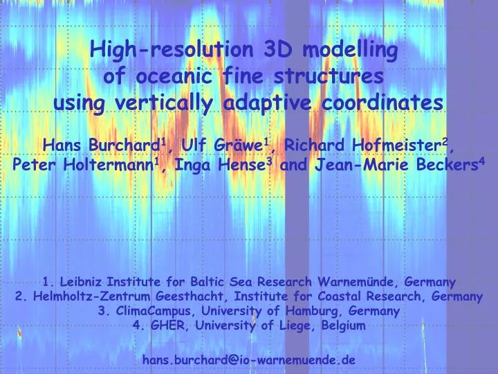
High-resolution 3D modelling of oceanic fine structures using vertically adaptive coordinates. Hans Burchard 1 , Ulf Gräwe 1 , Richard Hofmeister 2 , Peter Holtermann 1 , Inga Hense 3 and Jean-Marie Beckers 4 1. Leibniz Institute for Baltic Sea Research Warnemünde , Germany

E N D
High-resolution 3D modelling of oceanic fine structures using vertically adaptive coordinates Hans Burchard1, Ulf Gräwe1, Richard Hofmeister2, Peter Holtermann1, Inga Hense3 and Jean-Marie Beckers4 1. Leibniz Institute for Baltic Sea Research Warnemünde, Germany 2. Helmholtz-ZentrumGeesthacht, Institute for Coastal Research, Germany 3. ClimaCampus, University of Hamburg, Germany 4. GHER, University of Liege, Belgium hans.burchard@io-warnemuende.de
Representationofthinlayers in numericalmodels Thinlayerof material? Thinlayerof material Currentshear Patch of material Numerical grid Motivatedby Stacey et al. (2007)
Zooplankton migration in Central Baltic Sea Thereiscertainly a numericalproblemtobesolvedbeforewepredictthinlayers in 3D models.
Whatismixing ? Salinityequation (no horizontal mixing): Salinityvarianceequation: ? Mixing isdissipationoftracervariance.
Principleofnumericalmixingdiagnostics: First-order upstream (FOU) fors: 1D advectionequationforS: 1D advectionequationfors2: FOU forsisequivalenttoFOU fors²withvariancedecay: numericaldiffusivity Salinitygradientsquared See Maqueda Morales and Holloway (2006)
Generalisation by Burchard & Rennau (2008): Numerical variancedecayis … ( advected tracer square minus square of advected tracer) / Dt
„Baltic Slice“ simulation Burchard andRennau (2008)
salinity velocity numericalmixing physicalmixing Burchard andRennau (2008)
Verticallyintegratedsalinityvariancedecay Burchard andRennau (2008)
Hereistheproblem: Numerical mixingerodesstructureswhicharenumerically not well resolved, includingthinlayersverticallymovingwithinternalwaves. Neitherhighresolutionnor non-diffusiveadvectionschemes do efficientlysolvetheproblem. Whatcanbedone?
Adaptive vertical gridsin GETM Horizontal direction z hor. filteringof layer heights Vertical zooming of layer interfaces towards: a) Stratification b) Shear c) surface/ bottom hor. filteringof vertical position Lagrangiantendency Vertical direction isopycnaltendency Solution of a verticaldiffusionequation forthecoordinateposition bottom Hofmeister, Burchard & Beckers (2010a)
Baltic slice with adaptive verticalcoordinates Fixed coordinates Adaptive coordinates Hofmeister, Burchard & Beckers (2010)
Baltic slice with adaptive verticalcoordinates Hofmeister, Burchard & Beckers (2010)
Adaptive verticalcoordinates alongtransect in 600 m Western Baltic Sea model Gräwe et al. (in prep.)
1 nm Baltic Sea model with adaptive coordinates - refinement partially towards isopycnal coordinates - reduced numerical mixing - reduced pressure gradient errors - still allowing flow along the bottom salinity temperature km Hofmeister, Beckers & Burchard (2011)
Channelled gravitycurrent in Bornholm Channel sigma-coordinates - stronger stratification with adaptive coordinates- larger core of g.c. - salinity transport increased by 25% - interface jet along the coordinates adaptive coordinates Hofmeister, Beckers & Burchard (2011)
Gotland Sea time series • 3d baroclinic simulation • 50 adaptive layers vs. 50 sigma layers num. : turb. mixing 80% : 20% num. : turb. mixing 50% : 50% Hofmeister, Beckers & Burchard (2011)
Gotland Sea tracer release study thermocline halocline Holtermann et al. (in prep.)
Gotland Sea tracer release study Holtermann et al. (in prep.)
Gotland Sea tracer release study Grid adaptation to tracer concentration: Holtermann et al. (in prep.)
Annual North Seasimulationusing adaptive coordinates • 6 nmresolution • 30-50 vertical layers with a minimum thickness of 10 cm • adaptationtowardsstratification • adaptation towards nutrients and phytoplankton • productionrun 2005-2006 • NPZD included via FABM • NPZD starts 2005 from uniform values • open boundaries for FABM are taken from a 1D simulation of GOTM • hydrographic boundary conditions and atmospheric forcing are taken from the global NCEP CFSR runs (1/3o resolution FABM = Framework ofAquaticBiogeochamical Models (madebyJornBruggeman)
Ada Temperature in S1 [°C] phys & bio adaptive with 50 layers phys & bio adaptive with 30 layers phys adaptive with 30 layers non-adaptive with 30 layers Gräwe et al. (in prep.)
Layer thickness in S1 [m] phys & bio adaptive with 50 layers phys & bio adaptive with 30 layers phys adaptive with 30 layers non-adaptive with 30 layers Gräwe et al. (in prep.)
Physical mixing in S1 log10[Dphy/(K2/s)] phys & bio adaptive with 50 layers phys & bio adaptive with 30 layers phys adaptive with 30 layers non-adaptive with 30 layers Gräwe et al. (in prep.)
Numerical mixing in S1 log10[Dnum/(K2/s)] phys & bio adaptive with 50 layers phys & bio adaptive with 30 layers phys adaptive with 30 layers non-adaptive with 30 layers Gräwe et al. (in prep.)
Adaptation tobiogeochemicalproperties: Additionallytophysicalproperties (shearandstratification) diffusivitiesforgridlayerpositionequationarenow also composed of inverse valuesofbgcgradients such asnutrientand phytoplanktonconcentrationgradients. How strong theimpactofbgcgradientsisdepends on the individual weightingofthecomponents.
Nutrients at S1 [mmol N/m3] phys & bio adaptive with 50 layers phys & bio adaptive with 30 layers phys adaptive with 30 layers non-adaptive with 30 layers Gräwe et al. (in prep.)
Phytoplankton at S1 [mmol N/m3] phys & bio adaptive with 50 layers phys & bio adaptive with 30 layers phys adaptive with 30 layers non-adaptive with 30 layers Gräwe et al. (in prep.)
Phytoplankton at S1 log10[P/(mmol N/m3)] phys & bio adaptive with 50 layers phys & bio adaptive with 30 layers phys adaptive with 30 layers non-adaptive with 30 layers Gräwe et al. (in prep.)
Zooplankton at S1 [mmol N/m3] phys & bio adaptive with 50 layers phys & bio adaptive with 30 layers phys adaptive with 30 layers non-adaptive with 30 layers Gräwe et al. (in prep.)
Detritus at S1 [mmol N/m3] phys & bio adaptive with 50 layers phys & bio adaptive with 30 layers phys adaptive with 30 layers non-adaptive with 30 layers Gräwe et al. (in prep.)
Temperature along T1 [°C] phys & bio adaptive with 50 layers phys & bio adaptive with 30 layers phys adaptive with 30 layers non-adaptive with 30 layers Gräwe et al. (in prep.)
Physical mixing along T1 log10[Dphy/(K2/s)] phys & bio adaptive with 50 layers phys & bio adaptive with 30 layers phys adaptive with 30 layers non-adaptive with 30 layers Gräwe et al. (in prep.)
Nutrients along T1 [mmol N/m3] phys & bio adaptive with 50 layers phys & bio adaptive with 30 layers phys adaptive with 30 layers non-adaptive with 30 layers Gräwe et al. (in prep.)
Phytoplankton along T1 [mmol N/m3] phys & bio adaptive with 50 layers phys & bio adaptive with 30 layers phys adaptive with 30 layers non-adaptive with 30 layers Gräwe et al. (in prep.)
Zooplankton along T1 [mmol N/m3] phys & bio adaptive with 50 layers phys & bio adaptive with 30 layers phys adaptive with 30 layers non-adaptive with 30 layers Gräwe et al. (in prep.)
Conclusions Thinlayersaredifficulttorepresent in fixedverticalgrids … … unlessthethinlayersarethickorthenumberoflayersisextremelyhigh. Numericalmixing due toadvectionofbgcpropertiestendstoerodethinlayers, due tointernalwavesandtides. Neitherhighresolutionnorhigh-order advectionschemescanpreventthis. Adaptation ofverticallayerthicknessandpositiontolocationsofhighshear andstratificationmaysignificantlyimprovethesituation. The real solutionwouldbeverticalcoordinatesadaptingtobgcproperties. The nextstepwouldbetorealisticallysimulated a typicalthinlayerformation andmaintenancescenario in 3D, usingthisnewmethod.