Download
1 / 33
330 likes | 460 Views
V8 – 3D Modelling of TM proteins. Aim: structural modelling of G-protein coupled receptors. - involved in cell communication processes - mediate senses as vision, smell, taste, and pain - regulation of appetite, digestion, blood pressure, reproduction, inflammation Extracellular signals:

E N D
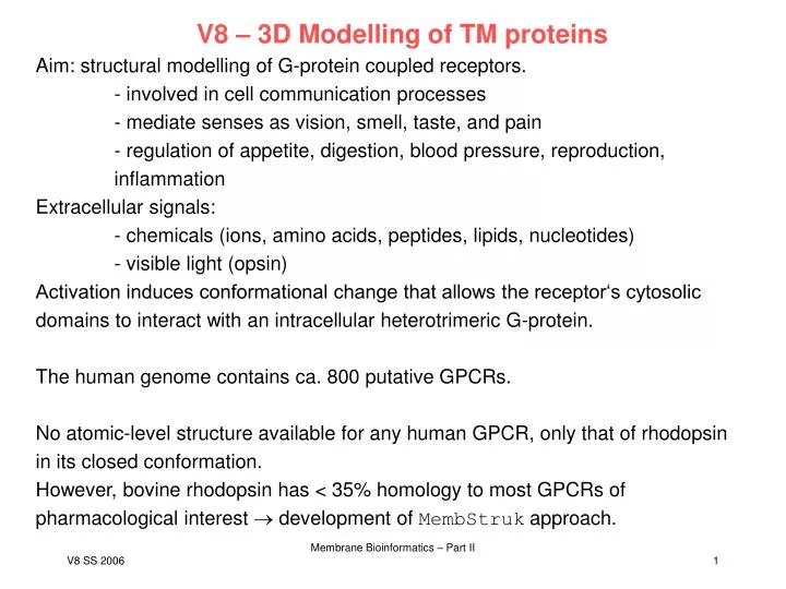
V8 – 3D Modelling of TM proteins Aim: structural modelling of G-protein coupled receptors. - involved in cell communication processes - mediate senses as vision, smell, taste, and pain - regulation of appetite, digestion, blood pressure, reproduction, inflammation Extracellular signals: - chemicals (ions, amino acids, peptides, lipids, nucleotides) - visible light (opsin) Activation induces conformational change that allows the receptor‘s cytosolic domains to interact with an intracellular heterotrimeric G-protein. The human genome contains ca. 800 putative GPCRs. No atomic-level structure available for any human GPCR, only that of rhodopsin in its closed conformation. However, bovine rhodopsin has < 35% homology to most GPCRs of pharmacological interest development of MembStruk approach. Membrane Bioinformatics – Part II
MembStruk Employ organizing principle: GPCRs have a single chain with 7 helical TM domains threading through the membrane. Overview: 1. Prediction of TM regions from analysis of the primary sequence 2. Assembly and coarse-grain optimization of the 7-helix TM bundle 3. Optimization of individual helices 4. Rigid-body dynamics of the helical bundle in a lipid bilayer 5. Addition of interhelical loops and optimization of the full structure. Membrane Bioinformatics – Part II
Step 1: Prediction of TM regions (TM2ndS) Assume that the outer regions of the TM helices (in contact with the hydrophobic tails of the lipid) should be hydrophobic, and that this character should be largest near the center of the membrane. 1a. Generate multiple sequence alignment. 1b. calculate consensus (average) hydrophobicity for every residue position in the alignment (Eisenberg hydrophobicity scale). Then calculate average hydrophobicity over a window size of 12-20 residues around every residue position. Plot average hydrophobicity at each position hydrophobicity profile. Membrane Bioinformatics – Part II
Step 1: Prediction of TM regions (TM2ndS) Fig. 1 shows that assigning the TM region to helix 7 is a problem because it has a shorter length and a lower intensity peak hydrophobicity compared with all the other helices. The low intensity of helix 7 arises because it has fewer highly hydrophobic residues (Ile, Phe, Val, and Leu) and because it has a consecutive stretch of hydrophilic residues (e.g., KTSAVYN). These short stretches of hydrophilic residues (including Lys-296) are involved in the recognition of the aldehyde group of 11-cis-retinal in rhodopsin. For such cases, we use the local average of the hydrophobicity (from minimum to minimum around this peak) as the baseline for assigning the TM predictions. TM2ndS automatically applies this additional criteria when the peak length is <23, the peak area is <0.8, and the local average >0.5 less than the base_mod. For bovine rhodopsin only TM7 satisfies this criterion and the local average (0.011) is shown by the red line in Fig. 1. Membrane Bioinformatics – Part II
Step 1: Helix capping 1c. It is possible that the actual length of the helix would extend past the membrane surface. Thus, we carry out a step aimed at capping each helix at the top and bottom of the TM domain. This capping step is based on properties of known helix breaker residues, but we restrict the procedure so as not to extend the predicted TM helical region more than six residues. We consider the potential helix breakers as P and G; positively charged residues as R, H, and K; and negatively charged residues as E and D. TM2ndS first searches up to four residues from the edge going inwards from the initial TM prediction obtained from the previous section for a helix breaker. If it finds one, then the TM helix edges are kept at the initial values. However, if no helix breaker is found, then the TM helical region is extended until a breaker is found, but with the restriction that the helix not be extended more than six residues on either side. The shortest helical assignment allowed is 21, corresponding to the shortest known helical TM region. This lower size limit prevents incorporation of narrow noise peaks into TM helical predictions. Membrane Bioinformatics – Part II
Step2: Assembly + optimization of the TM bundle 2a: Assembly of the 7 TM helices into a bundle. - construct canonical (ideal) -helices with extended side-chain conformations. - superimpose on 7.5 Å EM low-resolution structure of rhodopsin. No information on helix rotation angles. 2b. Optimize the relative translation of the helices in the bundle. - using remote homologous rhodopsin structure as basis for homology modelling would be risky - atomistic energy calculations may get trapped in local minima optimize packing by translating + rotating the helices by Monte-Carlo run. Membrane Bioinformatics – Part II
Step2: Assembly + optimization of the TM bundle 2b: ... assume that the mid point of the most hydrophobic helix stretch will be placed in the mid-plane of the bilayer: lipid midpoint plane (LMP). Membrane Bioinformatics – Part II
Step2c: Optimization of the rotational orientation Orienting the net hydrophobic moment of each helix to point toward the membrane (phobic orientation): In this procedure (denoted as CoarseRot-H), the helical face with the maximum hydrophobic moment is calculated for the middle section of each helix, denoted as the hydrophobic midregion (HMR). The face is the sector angle obtained as follows. 1), The central point of the sector angle is the intersection point of the helical axis (the active helix that is being rotated) with the common helical plane (LMP) and 2), the other two points forming the arc, are the nearest projections (on the LMP) of the Ca vectors of the two adjacent helices. The calculation of the hydrophobic moment vector is restricted to this face angle. This allows the predicted hydrophobic moment to be insensitive to cases in which the interior of the helix is uncharacteristically hydrophilic (because of ligand or water interactions within the bundle). Currently we choose HMR to be the middle 15 residues of each helix straddling the predicted hydrophobic center and exhibiting large hydrophobicity. This hydrophobic moment is projected onto the common helical plane (LMP) and oriented exactly opposite to the direction toward the geometric center of the TM barrel (GCB). This criterion is most appropriate for the six helices (excluding TM3) having significant contacts with the lipid membrane. The GCB is calculated as the center of mass of the positions of the -carbons for each residue in the HMR for each helix summed over all seven. Membrane Bioinformatics – Part II
Step2c: Optimization of the rotational orientation Optimization of the rotational orientation using energy minimization techniques (RotMin): each of the 7 TMs is optimized through a range of rotations and translations one at a time (the active TM) while the other six helices are reoptimized in response. After each rotation of the main chain (kept rigid) of each helix, the side-chain positions of all residues for all seven helices in the TMR are optimized (currently using SCWRL). The potential energy of the active helix is then minimized (for up to 80 steps of conjugate gradients minimization until an RMS force of 0.5 kcal/mol per Å is achieved) in the field of all other helices (whose atoms are kept fixed). This procedure is carried out for a grid of rotation angles (typically every 5° for a range of 50°) for the active helix to determine the optimum rotation for the active helix. Then we keep the active helix fixed in its optimum rotated conformation and allow each of the other six helices to be rotated and optimized. Here the procedure for each of the 6 helices one by one is 1), rotate the main chain; 2), SCWRL the side chains; and 3), minimize the potential energy of all atoms in the helix. The optimization of these 6 helices is done iteratively until the entire grid of rotation angles is searched. This method is most important for TM3, which is near the center of the GPCR TM barrel and not particularly amphipathic (it has several charged residues leading to a small hydrophobic moment). Membrane Bioinformatics – Part II
Step3: Optimizing the individual helices The optimization of the rotational and translational orientation of the helices described in the above steps is performed initially on canonical helices. To obtain a valid description of the backbone conformation for each residue in the helix, including the opportunity of G, P, and charged residues to cause a break in a helix, the helices built from the Step 2 were optimized separately. In this procedure, we first use SCWRL for side-chain placement, then carry out molecular dynamics (MD) (either Cartesian or torsional MD called NEIMO) simulations at 300 K for 500 ps, then choose the structure with the lowest total potential energy in the last 250 ps and minimize it using conjugate gradients. This optimization step is important to correctly predict the bends and distortions that occur in the helix due to helix breakers such as proline and the two glycines. The MD also carries out an initial optimization of the sidechain conformations, which is later further optimized within the bundle using Monte Carlo side-chain replacement methods. This procedure allows each helix to optimize in the field due to the other helices in the optimized TM bundle from Step 2. Membrane Bioinformatics – Part II
Step4: Addition of lipid bilayer and fine-grain reoptimization To the final structure from Step 3 MembStruk adds two layers of explicit lipid bilayers. This consists of 52 molecules of dilauroylphosphatidylcholine lipid around the TM bundle of seven helices. This was done by inserting the TM bundle into a layer of optimized bilayer molecules in which a hole was built for the helix assembly and eliminating lipids with bad contacts (atoms closer than 10 Å). Then we used the quaternion-based rigid-body molecular dynamics (RB-MD) in MPSim to carry out RB-MD for 50 ps (or until the potential and kinetic energies of the system stabilized). In this RB-MD step the helices and the lipid bilayer molecules were treated as rigid bodies and we used 1-fs time steps at 300 K. This RB-MD step is important to optimize the positions of the lipid molecules with respect to the TM bundle and to optimize the vertical helical translations, relative helical angles, and rotations of the individual helices in explicit lipid bilayers. Membrane Bioinformatics – Part II
Step5: loop building - Loops were added to the helices using WHATIF software. - use SCWRL to add side chains. - optimize loop conformations by conjugate gradient minimization of the loops while keeping TM helices fixed. This also allows forming selected disulfide linkages (e.g., between the cysteines in the EC-II loop, which are conserved across many GPCRs, and the N-terminal edge of TM3 or EC3). In the case of bovine rhodopsin, the alignment of the 44 sequences from Step 1, indicates only one pair of fully conserved Cys‘s on the same side of the membrane (extracellular side). The disulfide bond was formed and optimized with equilibrium distances lowered in decrements of 2 Å until the bond distance was itself 2 Å. Then the loop was optimized with the default equilibrium disulfide bond distance of 2.07 Å. - use annealing MD to optimize the EC-II loop. This involved 71 cycles, in each of which the loop atoms were heated from 50 K to 600 K and back to 50 K over a period of 4.6 ps. During this process the rest of the atoms were kept fixed for the first 330 ps and then the side chains within the cavity of the protein in the vicinity of the EC-II loop were allowed to move for 100 ps to allow accommodation of the loop. Subsequently a full-atom conjugate gradient minimization of the protein was performed in vacuum. This leads to the final MembStruk-predicted structure for bovine rhodopsin. Membrane Bioinformatics – Part II
Validation RMS difference between modelled and X-ray structure: 2.85 Å in the main-chain atoms 4.04 Å for all atoms in the TM helical region including loops: 6.80 Å RMSD in the main chain, 7.80 Å for all atoms. Correct loop modelling is very hard! Membrane Bioinformatics – Part II
PREDICT Starting basis: - homology models of GPCRs performed poorly in computational HT screening - diversity of ligand selectivity and signal transduction mechanisms appear to be caused by structural differences in the TM regions as well as in the extra- and intracellular domains. Here: develop de novo approach for modelling 3D structures of any GPCRs. Only consider physico-chemical properties of a single sequence. Membrane Bioinformatics – Part II
General Assumptions 1. The TMs are amphiphatic and have a length of 20–30 residues. 2. The loops connecting the helices are relatively short indicating that (a) the helices are packed in an antiparallel orientation and (b) the TMs are arranged in a sequential topology, so that the TM order along the sequence is also their order in the folded structure. 3. The TM helices are arranged in a counter-clockwise manner when viewed from the extracellular side as was shown for rhodopsin and bacteriorhodopsin. 4. Being embedded in a hydrophobic environment suggests that hydrophilic side-chains of the amphiphatic TM helices will favor the interior part of the protein, creating a “closed” structure in which the membrane-exposed surface is hydrophobic. Membrane Bioinformatics – Part II
Generate multiple decoys in 2D Step 1: determine the 7 TM domains. PREDICT uses a fuzzy identification of the helical domain. The actual TM domain is defined at a later stage. Then treat helices as 2D dials. Use simple geometrical rules to systematically generate all „reasonable“ close-packing conformations (decoys) in 2D. Assumption that the 7 helices form a closed structure of simple topology impose - the maximal diameter of the molecule must be < 5 the diameter of a single helix. - the maximal distance between two neighboring helices must be < 4 the diameter of a single helix. Use iterative grid search to systematically generate all 2D conformations of the 7 TMs that obey these rules. Grid search is conducted on the angles between every 3 adjacent helices (grid steps used as 15° (coarse search) or 6° (fine search)). It is possible to implement additional experimental knowledge. Membrane Bioinformatics – Part II
Optimizing Helical Rotational Orientation in 2D A common approach for orienting TM helices involves assigning a hydrophobicity moment to each TM helix. These vectors, which utilize various hydrophobicity scales, are then directed towards the lipid membrane orienting the helices accordingly. However, studies on membrane proteins demonstrated that hydrophobic moments are not sufficient for determining the solvent-accessible surface of TM helices. Aromatic-aromatic interactions are known to play a significant role in stabilizing both globular and membrane proteins. Some studies have indicated that more then 60% of Phe residues participate in aromatic stacking and about 80% of these involve more then two aromatic residues. Moreover, aromatic residues in alpha helices participate in both intrahelical and inter-helical interactions, thus affecting the rotational orientation of the TMs. PREDICT accounts for all these effects. Membrane Bioinformatics – Part II
From 2D dials to a reduced 3D structure (a) construct 3D-skeleton containing backbone atoms N, C and C. (b) use these coordinates as scaffold to construct reduced representation of the amino acid side chains. (c) use rotamer library to position full side chains Optimization of 3D structures (i) optimization of the vertical alignment of the helices relative to each other and to the membrane surface (ii) refinement of the inside-out distributions of the residues on each helix (iii) optimization of the position of the helix center in x-y plane (iv) assignment of helical tilt angles. Score optimized models according to their PREDICT energy score. Expansion to full atomistic models. Optimization with CHARMM force field (EM + MD). Membrane Bioinformatics – Part II
Application of modelled structures in drug design - construct 3D models of 5 different GPCRs - use DOCK4.0 to dock 1,600,000 drug-like compounds into 3D models - apply several scoring tools and selection criteria until a list of < 100 virtual hits is reached - automated binding-mode analysis - apply energy criteria (DOCK4.0, CHARMM) - filter by 3D-based principle component analysis with 5 – 50 descriptors only consider those compounds that fall within the same region as the known active compounds Membrane Bioinformatics – Part II
Application of modelled structures in drug design Membrane Bioinformatics – Part II
Application of modelled structures in drug design Certainly, modelled GPCR structures are not as accurate as X-ray structures. They are surprisingly powerful in enriching large ligand libraries. Novel binders can be detected. Membrane Bioinformatics – Part II
True de novo design We want to explore new TM protein topologies. Use efficient distance-dependent residue-residue force field to generate energetically favorable geometries of helix dimers. Assemble full protein structure from overlaying helix dimer geometries. Membrane Bioinformatics – Part II
docking of helix-dimers: energy scoring Example for parametrised energy function between 2 residues search 5 degrees of freedom systematically. score conformations by residue-residue energy function. Membrane Bioinformatics – Part II
docking of helix-dimers Test for Glycophorin A, dimer of two identical helices, structure known from NMR. • Energy landscape • around the minimum • Minimum is truly global minimum. RMSD between model and NMR structure only 0.8 Å. Membrane Bioinformatics – Part II
predicting the TM-helix-orientation from sequences CI: conservation index in multiple sequence alignment SASA: Solvent accessible surface area, relative to a single, free helix Test: correct orientation (0,0) has lowest score. fj(i): frequency of amino acid j in position i. fj : frequency of amino acid j in full alignment. C : mittlerer conservation index : Standardabweichung Positive values: conserved positions Negative values: variable positions result for 85 TM-helices helix-orientation can be predicted with an average error of 30° from the amino acid sequence alone. Membrane Bioinformatics – Part II
Ab initio structure prediction of TM bundles • Aim: construct structural model for a bundle of ideal transmembrane helices. • Construct 12 good geometries for every helix pair AB, BC, CD, DE, EF, FG • overlay ABCDEFG • „thinning out“ of solution space of 126 models • (a) remove „solutions“ where helices collide with eachother • (b) delete non-compact „solutions“ • score remaining 106 solutions by sequence conservation • cluster 500 best solutions in 8 models • rigid-body refinement, select 5 models with • best sequence conservation. Membrane Bioinformatics – Part II
compactness Membrane Bioinformatics – Part II
Rigid-body refinement Membrane Bioinformatics – Part II
Can one select the best model? • These are the four best non-native models of bR. • Because the contact between A and E was not imposed, very different topologies are obtained. • Currently, our methods cannot distinguish between these models. • they can serve as input for further experiments. Membrane Bioinformatics – Part II
Comparing the best models with X-ray structures dark: Model light: X-ray structure For (1) – (4) we used the known connectivity of the helices A-B-C-D-E-F-G. Otherwise, the search space would have been too large. Bakteriorhodopsin Halorhodopsin Sensory Rhodopsin Rhodopsin NtpK Membrane Bioinformatics – Part II
Comparing the best models with X-ray structures Membrane Bioinformatics – Part II
True de novo model Membrane Bioinformatics – Part II
Summary The basis for structure-based drug design is the availability of three-dimensional atomic protein structures. PREDICT and MembStruk methods provided good models for de novo drug design of potent binders. Typical steps of hierarchical modelling approaches: - identify TM domains - generate plausible low-resolution decoys - apply filters using compactness or hydrophobic moments - score by energy functions or by sequence conservation - add loops and generate atomistic models - refine using empirical force fields + MD simulations in explicit bilayers Potential of sequence conservation hasn‘t been fully exploited in the past. Membrane Bioinformatics – Part II