Download
1 / 40
400 likes | 483 Views
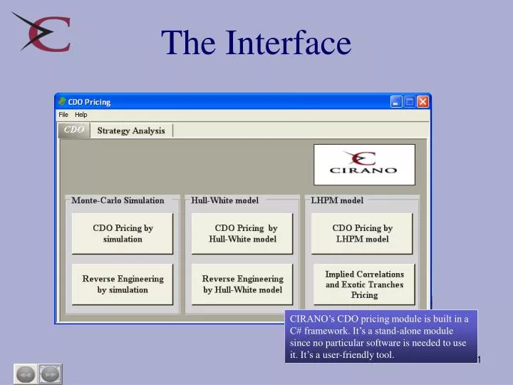
The Interface. CIRANO’s CDO pricing module is built in a C# framework. It’s a stand-alone module since no particular software is needed to use it. It’s a user-friendly tool. The Inputs. Let’s start with the « Evaluation » function of the Monte-Carlo simulations.

E N D
The Interface CIRANO’s CDO pricing module is built in a C# framework. It’s a stand-alone module since no particular software is needed to use it. It’s a user-friendly tool.
The Inputs Let’s start with the « Evaluation » function of the Monte-Carlo simulations. The user has to enter some of the main parameters of the CDO. The CDO maturity (in years), the payment frequency (usually quarterly) are examples of the required inputs. The current example uses a CDO with 10 collaterals. It’s possible to select a higher number of assets. However, this will cost more in terms of calculation time.
The Inputs The tranche to price has to be specified. The value, in millions of dollars, of the upper and lower boundaries have to be entered.
The Inputs Our module enables the use of specific data matrices. The files have to be in a text or spreadsheet format. The risk-free rate and an asset default correlation matrix are required. The value and the recovery rate of each asset are also inputs of the model.
The Inputs The term structure of the Credit Default Swap is also used in the model. It can be integrated through a external file or modelled with a Weibull function.
The Inputs It’s now time to simulate. The Quasi-Monte-Carlo technique has been added to our module. It generates the same results as a typical simulation while being more precise and requiring less simulations.
The Results Many interesting results come out of the simulations. The nominal value of the tranche is the first output given. The average upfrontspread (in % per year) is next. The upfront spread is the payment exceeding 500 basis points.
The Results The loss of the tranche during the given period is also available. So is its confidence interval. The loss dispersion statistics such as the standard deviation and the VaR are also displayed. All of these data are in basis points.
Sensitivity Analysis Once the results are obtained, it’s possible to perform sensitivity analyses. We want to determine the impact on the spread and on the loss of a 1 basis point decrease in the index.
Sensitivity Analysis Our results show that a 1 basis point decrease in the value of the index generates a 6.03 basis points spread increase and a loss of 0.338% on the value of the tranche.
The Interface The Hull and White model (2004) is an important feature of the CIRANO’s CDO pricing module. Major improvements have been realized in this module in regard to calculation time. It’s based on Gaussian copulas. The main characteristics of the CDO are in the upper section of the interface. These characteristics are the CDO maturity, the payment frequency and the number of assets.
The Inputs It’s important to mention that this model can price a CDO having 125 collaterals very quickly. It’s now also possible to price simultaneously all the tranches of the CDO without increasing the calculation time.
The Inputs Just like with the Monte-Carlo simulations, it’s possible to use external data matrices. These have to be in text or spreadsheet format. The following example will use Excel spreadsheets.
The Inputs The required inputs are mainly the same as the ones needed for the Monte-Carlo simulations. The correlation file is a vectorial file since the correlation is now calculated in regard to the market. The recovery rate is also fixed for all of the assets.
The Results • A few moments later, the results for the seven tranches appear. • Four important statistics are available for each tranche : • The upfront value of the spread (where applicable) • The Cherubini spread • The real spread • The nominal loss each tranche should suffer.
Sensitivity Analysis Just like with the Monte-Carlo simulations, spread and loss sensitivity analyses in regard to index or correlation movements can be perform. Here, we analyse the impact of a 1 basis point movement in the index.
Sensitivity Analysis To get an overview of the relationship the spread and the loss havewith the index or the correlation, graphics are generated. These are available for each of the analyses and can contain the value of one tranche or the values of all tranches.
The Interface Reverse engineering can be perform with the Monte-Carlo Simulations and the Hull and White model. This function makes it possible to find the implied correlation or the implied value of the index associated with the loss or the spread of a tranche.
The Inputs This example will perform reverse engineering with the Monte-Carlo simulations. The upfront value of the spread found in the previous Monte-Carlo example will be used to determine the implied correlation. The same inputs as the ones used for pricing are necessary.
The Results The implied correlation found with this upfront spread value is 0.3. This value is coherent with the one that has been used to simulate the spread in the previous example. Reverse engineering has then been efficiently performed.
The Interface The LHPM model may also be used to price CDO tranches.
The Inputs The LHPM model determines the prices of the tranches with the help of the base correlation of the CDO. It mainly uses the same inputs as the two previous pricing models.
The Inputs The model also uses the upfront value of the spread (represented by a 500 basis points value) for the appropriate tranches and the base correlation values of all the tranches.
The Results The following results are obtained : the fair spread, the upfront fee, the spread and the loss suffered by the tranche.
The Interface The LHPM model may also be used to determine the compound and implied correlations. It also prices exotic tranches.
The Inputs Using the spreads of the CDX tranches, it’s possible to compute the base correlation and compound correlation curves.
The Results Once the calculations are over, the values of the two types of correlation are obtained. Graphics display the associated curves.
Exotic Tranches Now that we have determine the base correlation curve, we are able to price exotic tranches with the LHPM model. This curve allows us to determine the base correlation value for a tranche having uncommon attachment point. To get this correlation, the button « Compute correlations » has to be pressed.
Exotic Tranches When we click on the « Tranche Pricing » button, the LPHM model and the base correlation previously found are used to determine the spread (in basis points and in upfront) of the exotic 0-2 tranche.
The Interface We have added to our module a CDO strategy analysis tool.
The Components At first, the historical values of the standard CDO tranches quotes and of the proper index have to be loaded into the module. An external file is used. Those tranches will be used to build the strategies.
The Components The user now has to build the strategy. The position on the tranche has to be specified (purchase or sale of protection) as well as the amount invested in each position (notional in millions of dollars).
The Components A few other inputs are necessary to perform the analysis of the strategy. Those inputs are fixed for all of the tranches.
Sensitivity Analysis We can now perform sensitivity analyses. One will study the value of the strategy following basis point changes in the value of the index spread and another will look at the strategy’s value after movements in the asset default correlation.
Sensitivity Analysis The results of the analyses are displayed in graphics. This one shows the marked-to-market value of our strategy following movements in the index spread.
Sensitivity Analysis A similar graphic shows the impacts on the strategy of changes in the asset default correlation.
Sensitivity Analysis It’s possible to look at the impacts of defaults on these sensitivity analyses. This kind of analysis can be performed by ticking the « One index type analysis » box and by choosing the number of defaults the CDO will suffer. If a strategy uses more than one standard CDO, the CDO suffering the defaults has to be specified.
Sensitivity Analysis The graphic we obtain is similar to the previous ones. However, an additional curve has been added. It represents the marked to market value of the strategy following a movement in the index spread in the case where 2 defaults have occurred.
Back-Testing The module enables the back-testing of the marked to market values of the strategy. Entry and exit dates are displayed for this analysis. By default, those dates are determined by the availability of the data contained in the file that has been loaded. They can be modified.
Back-Testing Following the analysis, this graphic is obtained.