Download
1 / 22
220 likes | 293 Views
ICOM 4075: Foundations of Computing. Lecture 8: Construction Techniques (1). Department of Electrical and Computer Engineering University of Puerto Rico at Mayagüez Summer 2005. Lecture Notes Originally Written By Prof. Yi Qian. Homework 7 (due Tuesday, April 6, 2010).

E N D
ICOM 4075: Foundations of Computing Lecture 8:Construction Techniques (1) Department of Electrical and Computer Engineering University of Puerto Rico at Mayagüez Summer 2005 Lecture Notes Originally Written By Prof. Yi Qian
Homework 7 (due Tuesday, April 6, 2010) • Section 2.3: (pp.111-115) 2. b. d. 3. b. 4. b. d. 5. b. d. f. h. 6. b. d. 7. b. d. 8. b. 9. b. d. f. 10. 14. 15. b.
Reading • Textbook: James L. Hein, Discrete Structures, Logic, and Computability, 2nd edition, Chapter 3. Section 3.1
Inductively Defined Sets • Definition of Inductive Definition • Example • A = {3, 5, 7, 9, …} • A = {2k + 3 | k N} • Another way to describe A is to observe that 3 A, that x A implies x + 2 A, and that the only way an element gets in A is by the previous two steps. This description has three ingredients, which we can state informally as follows: • 1. There is a starting element (3 in this case). • 2. There is a construction operation to build new elements from existing elements (addition by 2 in this case). • 3. There is a statement that no other elements are in the set. • An inductive definition of a set S consists of three steps: • Basic: Specify one or more elements of S. • Induction: Give one or more rules to construct new elements of S from existing elements of S. • Closure: State that S consists exactly of the elements obtained by the basis and induction steps. This step is usually assumed rather than stated explicitly.
Numbers • The set of natural numbers N = {0, 1, 2, …} is an inductive set. Its basis element is 0, and we can construct a new element from existing one by adding the number 1. So we can write an inductive definition for N in the following way. Basis: 0 N. Induction: if n N, then n + 1 N. • The constructors of N are the integer 0 and the operation that adds 1 to an element of N. The operation of adding 1 to n is called the successor function, which we write as succ(n) = n + 1 • Using the successor function, we can rewrite the induction step in the above definition of N in the alternative form If n N, then succ(n) N. • So we can say that N is an inductive set with two constructors, 0 and succ.
Some Familiar Odd Numbers • Give an inductive definition of A = {1, 3, 7, 15, 31, …}: • The basis case should place 1 in A. If x A, then we can construct another element of A with the expression 2x + 1. So the constructors of A are the number 1 and the operation of multiplying by 2 and adding 1. An inductive definition of A can be written as follows: Basis: 1 A. Induction: If x A, then 2x + 1 A.
Some Even and Odd Numbers • Is the following set inductive? A = {2, 3, 4, 7, 8, 11, 15, 16, …} It might be easier if we think of A as the union of the two sets B = {2, 4, 8, 16, …} and C = {3, 7, 11, 15, …}. Both these sets are inductive. The constructors of B are the number 2 and the operation of multiplying by 2. The constructors of C are the number 3 and the operation of adding by 4. We can combine these definitions to give an inductive definition of A. Basis: 2, 3 A. Induction: If x A and x is odd, then x + 4 A. If x A and x is even, then 2x A. This example shows that there can be more than one basis element, more than one induction rule, and tests can be included.
Strings • Let E denote the set of algebraic expressions, then we have the following inductive definition for E. Basis: If x is a variable or a number, then x E. Induction: If A, B E, then (A), A + B, A – B, AB, A B E. • Let’s recall that for an alphabet A, the set of all strings over A is denoted by A*. This set has the following inductive definition. • All Strings over A Basis: Λ A*. Induction: If s A* and a A, then as A*. • Note that when we place two strings next to each other in juxtaposition to form a new string, we are concatenating the two strings. So, from a computational point of view, concatenation is the operation we are using to construct new strings. • Recall that any set of strings is called a language. If A is an alphabet, then any language over A is one of the subsets of A*. Many languages can be defined inductively.
Three Languages • Many languages can be defined inductively. Here’re three examples. • 1. S = {a, ab, abb, abbb, …} = {abn | n N}. Informally, we can say that the strings of S consist of the letter a followed by zero or more b’s. But we can also say that the letter a is in S, and if x is a string in S, then so is xb. This gives us an inductive definition for S. Basis: a S. Induction: If x S, then xb S. • 2. S = {Λ, ab, aabb, aaabbb, …} = {anbn | n N}. Informally, we can say that the strings of S consist of any number of a’s followed by the same number of b’s. But we can also say that the empty string Λ is in S, and if x is a string in S, then so is axb. This gives us an inductive definition for S. Basis: Λ S. Induction: If x S, then axb S. • 3. S = {Λ, ab, abab, ababab, …} = {(ab)n | n N}. Informally, we can say that the strings of S consist of any number of ab pairs. But we can also say that the empty string Λ is in S, and if x is a string in S, then so is abx. This gives us an inductive definition for S. Basis: Λ S. Induction: If x S, then abx S.
Decimal Numerals • Recall that a decimal numeral is a nonempty string of decimal digits. For example, 2306 and 002576 are decimal numerals. If we let D denote the set of decimal numerals, we can describe D by saying that any decimal digit is in D, and if x is in D and d is a decimal digit, then dx is in D. This gives us the following inductive definition for D: Basis: {0, 1, 2, 3, 4, 5, 6, 7, 8, 9} D. Induction: If x D and d is a decimal digit, then dx D.
Lists • From a computational point of view the only parts of a nonempty list that can be accessed randomly are its head and its tail. • E.g., head(<x, y, z>) = x, and tail(<x, y, z>) = <y, z>. • The operation “cons” to construct lists: • E.g., cons(x, <y, z>) = <x, y, z>, cons(x, < >) = <x>. • The operations cons, head, and tail work nicely together. • E.g., we can write <x, y, z> = cons(x, <y, z>) = cons(head(<x, y, z>), tail(<x, y, z>)). • If L is any nonempty list, then we have the equation L = cons(head(L), tail(L)). • To write an inductive definition for lists(A): • Informally, we can say that lists(A) is the set of all ordered sequences of elements taken from the set A. But we can also say that < > is in lists(A), and if L is in lists(A), then so is cons(a, L) for any a in A. This gives us an inductive definition for lists(A), whixh can state formally as follows: All Lists over A: Basis: < > lists(A). Induction: If x A and L lists(A), then cons(x, L) lists(A).
List Membership • Let A = {a, b}. We’ll use the inductive definition for lists(A) to show how some lists become members of lists(A). The basis case puts < > lists(A). Since a A and < > lists(A), the induction step gives <a> = cons(a, < >) lists(A). In the same way we get <b> lists(A). Now since a A and <a> lists(A), the induction step puts <a, a> lists(A). Similarly, we get <b, a>, <a, b>, and <b, b> as elements of lists(A), and so on.
A Notational Convenience • It’s convenient when working with lists to use an infix notation for cons to simplify the notation for list expressions. We’ll use the double colon symbol ::, so that the infix form of cons(x, L) is x :: L. • E.g., the list <a, b, c> can be constructed using cons as cons(a, cons(b, cons(c, < >))) = cons(a, cons(b, <c>)) = cons(a, <b, c>) = <a, b, c>. Using the infix form, we construct <a, b, c> as follows: a :: (b :: (c :: < >)) = a :: (b :: <c>) = a :: <b, c> = <a, b, c>. • The infix form of cons allows us to omit parentheses by agreeing that :: is right associative. In other words, a :: b :: L = a :: (b :: L). Thus we can represent the list <a, b, c> by writing a :: b :: c :: < > instead of a :: (b :: (c :: < >)). • Many programming problems involve processing data represented by lists. The operations cons, head, and tail provide basic tools for writing programs to create and manipulate lists. So they are necessary for programmers.
Lists of Binary Digits • Suppose we need to define the set S of all nonempty lists over the set {0, 1} with the property that adjacent elements in each list are distinct. We can get an idea about S by listing a few elements: S = {<0>, <1>, <1, 0>, <0, 1>, <0, 1, 0>, <1, 0, 1>, …}. Let’s try <0> and <1> as basis elements of S. Then we can construct a new list from a list L S by testing whether head(L) is 0 or 1. If head(L) = 0, then we place 1 at the left of L. Otherwise, we place 0 at the left of L. So we can write the following inductive definition for S. Basis: <0>, <1> S. Induction: If L S and head(L) = 0, then cons(1, L) S. If L S and head(L) = 1, then cons(0, L) S. The infix form of this induction rules looks like If L S and head(L) = 0, then 1 :: L S. If L S and head(L) = 1, then 0 :: L S.
Lists of Letters • Suppose we need to define the set S of all lists over {a, b} that begin with the single letter a followed by zero or more occurrences of b. We can describe S informally by writing a few of its elements: S = {<a>, <a, b>, <a, b, b>, <a, b, b, b>, …}. It seems appropriate to make <a> the basis element of S. Then we can construct a new list from any list L S by attaching the letter b on the right end of L. But cons places new elements at the left end of a list. We can overcome the problem in the following way: If L S, then cons(a, cons(b, tail(L)) S. In infix form the statement reads as follows: If L S, then a :: b :: tail(L) S. For example, if L = <a>, then we construct the list a :: b :: tail(<a>) = a :: b :: < > = a :: <b> = <a, b>. So we have the following inductive definition of S: Basis: <a> S. Induction: If L S, then a :: b :: tail(L) S.
All Possible Lists • To find an inductive definition for the set of all possible lists over {a, b}, including lists that can contain other lists: Suppose we start with lists having a small numbers of symbols, including the symbols < and >. Then for each n ≥ 2, we can write down the lists made up of n symbols (not including commas). The figure in the following shows these listings for the first few values of n. If we start with the empty list < >, then with a and b we can construct three more lists as follows: a :: < > = <a>, b :: < > = <b>, < > :: < > = << >>. Now if we take these three lists together with < >, then with a and b we can construct many more lists. For example, a :: <a> = <a, a>, <a> :: < > = <<a>>, << >> :: <b> = <<< >>, b>, <b> :: << >> = <<b>, < >>. Using this idea, we’ll make an inductive definition for the set S of all possible lists over A: Basis: < > S. Induction: If x A S and L S, then x :: L S. • 3 4 5 6 • < > <a> << >> <<a>> <<< >>> • <b> <a, a> <<b>> << >, < >> • <a, b> << >, a> <a, a, < >> • <b, a> << >, b> <a, < >, a> • <b, b> <a, < >> << >, a, a> • <b, < >> <a, b, < >> • <a, a, a> <a, b, a, b> • … … … …
Binary Trees • In Chapter 1 we represented binary trees by lists, where the empty binary tree is denoted by < > and a nonempty binary tree is denoted by the list <L, x, R>, where x is the root, L is the left subtree, and R is the right subtree. This gives us the ingredients for a more formal inductive definition of the set of all binary trees. • For convenience we’ll let tree(L, x, R) denote the binary tree with root x, left subtree L, and right subtree R. If we still want to represent binary trees as tuples, then of course we can write tree(L, x, R) = <L, x, R>. • Now suppose A is any set. Then we can describe the set B of all binary trees whose nodes come from A by saying that < > is in B, and if L and R are in B, then so is tree(L, a, R) for any a in A. This gives us an inductive definition, which we can state formally as follows. • All Binary Trees over A: Basis: < > B. Induction: If x A and L, R B, then tree(L, x, R) B. • We also have destructor operations for binary trees. We’ll let left, root, and right denote the operations that return the left subtree, the root, and the right subtree, respectively, of a nonempty tree. • E.g., if T = tree(L, x, R), then left(T) = L, root(T) = x, and right(T) = R. So for any nonempty binary tree T we have T = tree(left(T), root(T), right(T)).
0 0 1 1 0 0 1 1 1 1 Binary Trees of Twins • Let A = {0, 1}. Suppose we need to work with the set Twins of all binary trees T over A that have the following property: The left and right subtrees of each node in T are identical in structure and node content. For example, Twins contains the empty tree and any single-node tree. Twins also contains the two trees shown in the following Figure. • We can give an inductive definition of Twins by simply making sure that each new tree has the same left and right subtree. Here’s the definition: Basis: < > Twins. Induction: If x A and T Twins, then tree(T, x, T) Twins.
1 0 1 0 0 1 0 1 1 0 Binary Trees of Opposites • Let A = {0, 1}, and suppose that Opps is the set of all nonempty binary trees T over A with the following property: The left and right subtrees of each node of T have identical structures, but the 0’s and 1’s are interchanged. For example, the single node trees are in Opps, as well as the two trees shown in the Figure in the following. • Since our set does not include the empty tree, the two singleton trees with nodes 1 and 0 should be the basis trees in Opps. The inductive definition of Opps can be given as follows: Basis: tree(< >, 0, < >), tree(< >, 1, < >) Opps. Induction: Let x A and T Opps. If root(T) = 0, then tree(T, x, tree(right(T), 1, left(T))) Opps. Otherwise, tree(T, x, tree(right(T), 0, left(T))) Opps.
y + 1 y x x + 1 Cartesian Products of Sets • Consider the problem of finding inductive definitions for subsets of the Cartesian product of two sets. For example, the set N x N can be defined inductively by starting with the pair (0, 0) as the basis element. Then, for any pair (x, y) in the set, we can construct the following three pairs. (x + 1, y + 1), (x, y + 1), and (x + 1, y). The graph in the following shows an arbitrary point (x, y) together with the three new points. It seems clear that this definition will define all elements of N x N, although some points will be defined more than once. For example, the point (1, 1) is constructed from the basis element (0, 0), but it is also constructed from the point (0, 1) and the point (1, 0). • Cartesian Product: A Cartesian product can be defined inductively if at least one of the sets in that product can be inductively. For example, if A is any set, then we have the following inductive definition of N x A: Basis: (0, a) N x A for all a A. Induction: If (x, y) N x A, then (x + 1, y) N x A.
Part of a Plane • Let S = {(x, y) | x, y N and x ≤ y}. From the point of view of a plane, S is the set of points in the first quadrant with integer coordinates on or above the main diagonal. We can define S inductively as follows: Basis: (0, 0) S. Induction: If (x, y) S, then (x, y + 1), (x + 1, y + 1) S. For example, we can use (0, 0) to construct (0, 1) and (1, 1). From (0, 1) we can construct (0, 2) and (1, 2). From (1, 1) we construct (1, 2) and (2, 2). So some pairs get defined more than once.
f(x) f A x a b Describing an Area • We can think of a area as a set of ordered pairs (x, y) forming a subset of N x N : • Describe the area A under the curve of a function f between two points a and b on the x-axis (see the Figure). The area A can be described as the following set of points: A = {(x, y) | x, y N, a ≤ x ≤ b, and 0 ≤ y ≤ f(x)}. • There are several ways to give an inductive definition of A. For example, we can start with the points (a, 0) on the x-axis. From (a, 0) we can construct the column of points above it and the point (a + 1, 0), from which the next column of points can be constructed. Here’s the definition: Basis: (a, 0) A. Induction: If (x, 0) A and x < b, then (x + 1, 0) A. If (x, y) A and y < f(x), then (x, y + 1) A. • For example, the column of points (a, 0), (a, 1), (a, 2), …, (a, f(a)) is constructed by starting with the basis point (a, 0) and by repeatedly using the second if-then statement. The first if-then statement constructs the points on the x-axis that are then used to construct the other columns of points. Notice with this definition that each pair is constructed exactly once.