Download
1 / 17
170 likes | 292 Views
What Types Of Data Are Collected?. Research Is A Partnership Of Questions And Data. “Categorical” Data. “Continuous” Data. S010Y: Answering Questions with Quantitative Data Class 5/II.2: Examining the Relationship Between Categorical Variables.

E N D
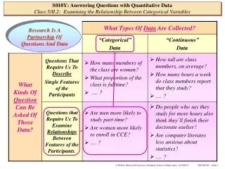
What Types Of Data Are Collected? Research Is A Partnership Of Questions And Data “Categorical” Data “Continuous” Data S010Y: Answering Questions with Quantitative DataClass 5/II.2: Examining the Relationship Between Categorical Variables What Kinds Of Question Can Be Asked Of Those Data? Questions That Require Us To Describe Single Features of the Participants • How many members of the class are women? • What proportion of the class is fulltime? • …. ? • How tall are class members, on average? • How many hours a week do class members report that they study? • …. ? Questions that Require Us To Examine Relationships Between Features of the Participants. • Are men more likely to study part-time? • Are women more likely to enroll in CCE? • …. ? • Do people who say they study for more hours also think they’ll finish their doctorate earlier? • Are computer literates less anxious about statistics? • …. ?
In other words, we are being asked whether the values in theDEATHcolumn correspond to the values in theRVICTIMcolumn in some meaningful way? • Our approach: • Display the sample relationship between DEATH and RVICTIM in a “two-way contingency table.” • Describe their sample relationship with suitable sample percentages. • Summarize their sample relationship using a Pearson Chi-square (2) statistic. • Use statistical inference to carry out a statistical test? • Interpret and tell the story (especially to Justice Powell). And, as we’ve seen, this question can be addressed in the DEATHPEN dataset, by asking whether categorical variable DEATH is related to categorical variable RVICTIM, in the sample of convicted murderers. 0 1 1 0 1 1 0 1 1 0 1 1 0 1 1 . (2475 cases) . 1 2 2 1 2 2 1 2 2 We’re trying to address the following research question: Is it more probable that a convicted murderer will be sentenced to death, in Georgia, if he kills someone Black, or if he kills someone White? S010Y: Answering Questions with Quantitative DataClass 5/II.2: Examining the Relationship Between Categorical Variables
Frequencies we haveobservedin the sample … So far, we’ve begun by displaying and describing the sample relationship in a two-way contingency table: Our prior estimation of slice-by-slicepercentages in this block chart has described the sample relationship between DEATH and RVICTIM in these data. S010Y: Answering Questions with Quantitative DataClass 5/II.2: Examining the Relationship Between Categorical Variables • For instance, • When the victim was Black, 1.33% of defendants were sentenced to death. • When the victim was White, 11.1% of the defendants were sentenced to death. • So, the percentage of our sample of convicted murderers who were sentenced to death in Georgia after killing a White victim was 8.33 times the percentage of convicted murderers who were sentenced to death after killing a Black victim. This descriptive analysis suggests that knowing the value of RVICTIM does indeed help you predict the value of DEATH, in the sample, andso perhaps we might legitimately conclude that DEATH and RVICTIM are “related.”
And then we asked ourselves how different the observed and expected tables of sample frequencies are? • If the “observed” and “expected” contingency tables seem very similar, we might be tempted to conclude that we have not observed much of a relationship between DEATH & RVICTIM, or that it is even zero?? • If the “observed” and “expected” contingency tables seem very different from each other, we might be tempted to say that a relationship does indeed exist between the variables, and may be quite strong???? To help summarize the sample relationship betweenDEATH&RVICTIM more fully, we imagined what the sample might look like if there were no relationship between the two variables, as follows: S010Y: Answering Questions with Quantitative DataClass 5/II.2: Examining the Relationship Between Categorical Variables
It was called the Pearson 2 statistic: To help us in our quest to computerize this process, we summarized the net discrepancy between the tables of observed and expectedfrequencies by estimatinga single number index ... S010Y: Answering Questions with Quantitative DataClass 5/II.2: Examining the Relationship Between Categorical Variables
Key Issues: • What is “big”? • What is “close to zero”? • Is 115big or close to zero? “If 2 is big, then declare that there is a relationship between DEATH and RVICTIM” Decision Rule??? “If 2 is zero, orclose to zero, then declare there is no relationship between DEATH and RVICTIM” S010Y: Answering Questions with Quantitative DataClass 5/II.2: Examining the Relationship Between Categorical Variables
Thisprocess of generalization is called statistical inference. It is central to quantitative methods! To respond to these issues we must step back … and think more broadly about the nature of the problem we’re facing … • First, let’s re-assess where we are … • All we’ve done so far is putter around in somedata on asample of convicted murderers. • But. out there, somewhere, let’s assume there’s alarger population of convicted murderersfrom which our sample was drawn. • Is there some aspect of this “sampling from a population” that could help us resolve our problem? • And, wouldn’t our conclusions be more compelling if there was some way to generalize our sample conclusions about the DEATH-RVICTIM relationship back to the underlying population. S010Y: Answering Questions with Quantitative DataClass 5/II.2: Examining the Relationship Between Categorical Variables
Of course … when you generalize from a sample back to its underlying population, you must be careful that your sole original empirical findinghas not been thevictim of sampling idiosyncrasy!!! • For instance, could the following scenario be plausible? • What if there is really no relationshipbetween DEATH and RVICTIM in the underlying population? • But in our research, by an accident of sampling, we just happen to have drawn an odd-ball sample from this population. • And it is this “sampling idiosyncrasy” that has ended up giving us a 2 statistic as large as 115, but it is purely by accident. S010Y: Answering Questions with Quantitative DataClass 5/II.2: Examining the Relationship Between Categorical Variables If this could have happened, we wouldn’t want to claim a relationship between DEATH and RVICTIMdespite the sample evidence to the contrary!! How Can We Assess The Plausibility Of Such A Scenario?
Sample #1, 2 = 3.2 Sample #2, 2 = 0.3 Etc. Sample #3, 2 = 17.4 Etc. Hypothetical Scenario… let’s imagine that we could draw samples of 2475 murderers repeatedly from a hypothetical population of convicted murderers in which there really was no relationship between DEATH & RVICTIM … in each case, we could go ahead and estimate the 2 statisticfor each drawing,using our usual methods !! S010Y: Answering Questions with Quantitative DataClass 5/II.2: Examining the Relationship Between Categorical Variables Hypothetical “Null Population” in which: H0: DEATH & RVICTIM are not related
Frequency of occurrence of each accidental value of the Pearson 2 Statistic Accidental value of the Pearson 2 Statistic 0 10 20 30 40 50 60 70 80 90 100 110 120 130 140 115 If such a histogram were available, it would give us the perfect context for deciding whether our sole “empirical” value of the 2 statistic (of 115) was “big” or “small”!!! In this hypothetical “repeated sampling from a null population” scenario, we could then record all the values of the 2 statistic that we obtained, in a vertical histogram… What If Such A Set Of Samplings From A Hypothetical Null Population Produced A Vertical Histogram That Looked Like This? S010Y: Answering Questions with Quantitative DataClass 5/II.2: Examining the Relationship Between Categorical Variables Histogram summarizes the “natural variation” that might occur in the Pearson 2 statistic as a result of sampling idiosyncrasy, if we were to repeatedly draw samples from a hypothetical population in which there is no relationship between DEATH and RVICTIM.
Frequency of occurrence of each accidental value of the Pearson 2 Statistic Accidental value of the Pearson 2 Statistic 0 10 20 30 40 50 60 70 80 90 100 110 120 130 140 115 What If Such A Set Of Samplings From A Hypothetical Null Population Produced A Vertical Histogram That Looked Like This? S010Y: Answering Questions with Quantitative DataClass 5/II.2: Examining the Relationship Between Categorical Variables If This Were The Histogram That Could Be Obtained From A Hypothetical Null Population By Sampling Idiosyncrasy, What Would You Think Of Our Actual Value Of 115?
“Hey, in a hypothetical exercise of sampling repeatedly from a null population, 0.9999 of all accidental values of the 2 statistic are going to fall to the left of a value of 115!!!” Or, … “Hey, in a hypothetical exercise of sampling repeatedly from a null population, only 0.0001 of all accidental values of the 2 statistic are going to fall to the right of a value of 115!!! Frequency of occurrence of each accidental value of the Pearson 2 Statistic Accidental value of the Pearson 2 Statistic 0 10 20 30 40 50 60 70 80 90 100 110 120 130 140 Actually, for you to reach a conclusion, I wouldn’t really even have to show you the entire vertical histogram … I could just tell you one of the two following alternatives … What If Such A Set Of Samplings From A Hypothetical Null Population Produced A Vertical Histogram That Looked Like This? S010Y: Answering Questions with Quantitative DataClass 5/II.2: Examining the Relationship Between Categorical Variables 115 • In fact, I really only need to tell you one of these stories … so, I choose to tell you the one on the right: • “In repeated sampling from a null population, we’d expect the proportion of all of the accidental values of the Pearson 2 statistic that could be equal to, or greater than, 115 by an accident of sampling, to be .0001” We call this proportion, the “p-value.” It can be obtained by computer simulation, or from tables.
At what p-valuewould you cease to believe that the single value of the 2 statistic that you had obtained in your actual empirical researchwas “big” .001 .10 .05 .01 .0001 .25 .50 S010Y: Answering Questions with Quantitative DataClass 5/II.2: Examining the Relationship Between Categorical Variables Sole Value of Your Statistic Sole Value of Your Statistic Sole Value of Your Statistic Sole Value of Your Statistic Sole Value of Your Statistic Sole Value of Your Statistic Sole Value of Your Statistic
This is the usual titling, data input, labeling and formatting that you have seen several times – it should be getting quite familiar by now Next page.. Of course, we can’t actually do all this random re-sampling from a hypothetical null population … but we can get the computer to simulate it and tell us what it finds … it’s in Class 5/Handout 1 OPTIONS Nodate Pageno=1; TITLE1 'A010Y: Answering Questions with Quantitative Data'; TITLE2 'Class 5/Handout 1: Introducing the Notion of Statistical Inference'; TITLE3 'Death penalty and race bias in Georgia'; TITLE4 'Data in DEATHPEN.txt'; *-------------------------------------------------------------------------* Input data, name and label variables in dataset *-------------------------------------------------------------------------*; DATA DEATHPEN; INFILE 'C:\DATA\A010Y\DEATHPEN.txt'; INPUT DEATH RDEFEND RVICTIM; LABEL DEATH = 'Sentenced to death?' RDEFEND = 'Race of defendant' RVICTIM = 'Race of victim'; *-------------------------------------------------------------------------* Format labels for values of categorical variables *-------------------------------------------------------------------------*; PROC FORMAT; VALUE DFMT 0 = 'No' 1 = 'Yes'; VALUE RFMT 1 = 'Black' 2 = 'White'; *-------------------------------------------------------------------------* Summarizing the relationship between DEATH and RVICTIM *-------------------------------------------------------------------------*; PROC FREQ DATA=DEATHPEN; TITLE5 'Using a p-value to Test the Relationship Between DEATH and RVICTIM'; FORMAT DEATH DFMT. RVICTIM RFMT.; TABLES DEATH*RVICTIM / EXPECTED DEVIATION CELLCHI2 CHISQ NOCOL NOROW NOPERCENT; RUN; S010Y: Answering Questions with Quantitative DataClass 5/II.2: Examining the Relationship Between Categorical Variables
PC_SAS uses the PROCFREQ procedure to carry out standard contingency table analyses. TheTABLEScommand requests a contingency table of DEATH by RVICTIM. TheEXPECTEDoption requests the computation of the expected frequencies. The DEVIATIONoption requests the computation of the difference between the observed and expected frequencies. TheCELLCHISQoption requests the computation of the bit of the overall 2 statistic that is contributed by each cell in the contingency table. The CHISQoption requests the estimation of the 2 statistic. S010Y: Answering Questions with Quantitative DataClass 5/II.2: Examining the Relationship Between Categorical Variables *-------------------------------------------------------------------------------* Summarizing the relationship between DEATH and RVICTIM *-------------------------------------------------------------------------------*; PROC FREQ DATA=DEATHPEN; TITLE5 'Using a p-value to Test the Relationship Between DEATH and RVICTIM'; FORMAT DEATH DFMT. RVICTIM RFMT.; TABLES DEATH*RVICTIM / EXPECTED DEVIATION CELLCHI2 CHISQ NOCOL NOROW NOPERCENT; RUN;
Here’s the observed frequency in the cell Here’s the expected frequency in the cell Here’s the observed frequency minus the expected frequency in the cell Here’s the cell’s contribution to the 2 statistic Here the 2 statistic, 114.9 Here’s the p-value, < .0001 Because thep-value is less than .05 (representing a 5% chance of getting this a 2 statistic this large by anaccident of samplingfrom anull population), we can conclude thatDEATHandRVICTIMare relatedin the actual population of convicted murderers in Georgia … S010Y: Answering Questions with Quantitative DataClass 5/II.2: Examining the Relationship Between Categorical Variables
So, there it is … Statistical Inference… in several very tortuous steps: • State a Research Question: Is imposition of the death penalty related to the race of the victim in the population of convicted murderers in Georgia? • Display and Describe the Observed Data:use a block chart and sample frequencies. • Summarize the Observed Data in a Contingency Table: find the observed frequencies, figure out expected frequencies, estimate the 2 statistic. • Obtain the p-value: figure out how likely it is that you could’ve obtained a value of the 2 statistic equal to, or greater than, the observed valueby an accident of sampling from a population in which the null hypothesis(i.e., a population in which the statement “H0: DEATH & RVICTIM are not related” is true). • If Your p-value Is Less Than .05 (.01? .10?), Reject the Null Hypothesisand conclude that there really is a relationship between DEATH and RVICTIMin the population – i.e., that you are confident your finding is not a consequence of idiosyncratic sampling. • Interpret Your Findings In Words, Drawing Explicitly On Your Plots, Summary Statistics and Test Statistics, for a naïve but intelligent audience to read. S010Y: Answering Questions with Quantitative DataClass 5/II.2: Examining the Relationship Between Categorical Variables “In the population of convicted murderers in Georgia, capital sentencing and race of victim are related (2 = 115, p < .0001). The percentage of convicted murderers who were sentenced to death after killing a White victim was more than 8 times the percentage of convicted murderers who were sentenced to death after killing a Black victim. In the block chart in Figure 1, notice that … etc.” p.s. Make sure the Supreme Court gets the memo!