Download
1 / 44
440 likes | 619 Views
The Gravitomagnetic effect measurement ( Creditis to Davide Lucchesi ). Table of Contents. Gravitomagnetism and Lense–Thirring effect; The LAGEOS satellites and SLR; The 2004 measurement and its error budget (EB);

E N D
The Gravitomagnetic effect measurement(Creditis to Davide Lucchesi)
Table of Contents • Gravitomagnetism and Lense–Thirring effect; • The LAGEOS satellites and SLR; • The 2004 measurement and its error budget (EB); • Difficulties in improving the present measurement with LAGEOS satellites only; • Conclusions;
Gravitomagnetism and Lense–Thirring effect It is interesting to note that, despite the simplicity and beauty of the ideas of Einstein’s GR, the theory leads to very complicated non–linear equations to be solved: these are second–order–partial–differential–equations in the metric tensor g, i.e., hyperbolic equations similar to those governing electrodynamics. However, we can find very interesting solutions, removing at the same time the mathematical complications of the full set of equations, in the so–called weak field and slow motion (WFSM) limit . Under these simplifications the equations reduce to a form quite similar to those of electromagnetism.
Gravitomagnetism and Lense–Thirring effect This leads to the “ Linearized Theory of Gravity ”: Flat spacetime metric: gauge conditions; metric tensor; field equations; and h represents the correction due to spacetime curvature where weak field means h« 1; in the solar system where is the Newtonian or “gravitoelectric” potential:
Gravitomagnetism and Lense–Thirring effect are equivalent to Maxwell eqs.: That is, the tensor potential plays the role of the electromagnetic vector potential A and the stress energy tensor T plays the role of the four–current j. represents the solution far from the source: (M,J) gravitoelectric potential; gravitomagnetic vector potential; J represents the source total angular momentum or spin
Gravitomagnetism and Lense–Thirring effect Following this approach we have a field, the Gravitoelectric field produced by masses, analogous to the electric field produced by charges: and a field, the Gravitomagnetic field produced by the flow of matter, i.e., mass–currents, analogous to the magnetic field produced by the flow of charges, i.e., by electric currents: This is a crucial point and a way to understand the phenomena of GR associated with rotation, apparent forces in rotating frames and the origin of inertia in general.
Gravitomagnetism and Lense–Thirring effect These phenomena have been debated by scientists and philosophers since Galilei and Newton times. In classical physics, Newton’s law of gravitation has a counterpart in Coulomb’s law of electrostatics, but it does not have any phenomenon formally analogous to magnetism. On the contrary, Einstein’s theory of gravitation predicts that the force generated by an electric current, that is Ampère’s law of electromagnetism, should have a formal counterpart force generated by a mass–current.
h(r) BG(r) A(r) B(r) r r J Jm Je Gravitomagnetism and Lense–Thirring effect The Analogy Classical electrodynamics: Classical geometrodynamics: G = c = 1
B BG ’ S J Gravitomagnetism and Lense–Thirring effect The Analogy G = c = 1 This phenomenon is known as the “dragging of gyroscopes” or “inertial frames dragging” This means that an external current of mass, such as the rotating Earth, drags and changes the orientation of gyroscopes, and gyroscopes are used to define the inertial frames axes.
Gravitomagnetism and Lense–Thirring effect In GR the concept of inertial frame has only a local meaning: they are the frames where locally, in space and time, the metric tensor (g) of curved spacetime is equal to the Minkowski metric tensor () of flat spacetime: And a local inertial frame is ‘’rotationally dragged‘’ by mass-currents, i.e., moving masses influence and change theorientation of the axes of a local inertial frame (that is of gyroscopes);
Schwarzschild metric which gives the field produced by a non–rotating massive sphere Kerr metric which gives the field produced by a rotating massive sphere Gravitomagnetism and Lense–Thirring effect The main relativistic effects due to the Earth on the orbit of a satellite come from Earth’s mass M and angular momentum J. In terms of metric they are described by Schwarzschild metric and Kerr metric:
Angular momentum Gravitomagnetism and Lense–Thirring effect Secular effects of the Gravitomagnetic field: Rate of change of the ascending node longitude: (Lense–Thirring, 1918) Rate of change of the argument of perigee: These are the results of the frame–dragging effect or Lense–Thirring effect: moving masses (i.e., mass–currents) are rotationally dragged by the angular momentum of the primary body (mass–currents)
Gravitomagnetism and Lense–Thirring effect Z Orbital plane Equatorial plane semimajor axis; eccentricity; inclination; I longitude of the ascending node; argument of perigee; mean anomaly; Y X Ascending Node direction L Epoch Orbital Inclination Right Ascension of Ascending Node (R.A.A.N.) Argument of Perigee Eccentricity Mean Motion Mean Anomaly Keplerian elements
The LT effect on LAGEOS and LAGEOS II orbit Rate of change of the ascending node longitude and of the argument of perigee : LAGEOS: LAGEOS II: 1 mas/yr = 1 milli–arc–second per year 30 mas/yr 180 cm/yr at LAGEOS and LAGEOS II altitude
Table of Contents • Gravitomagnetism and Lense–Thirring effect; • The LAGEOS satellites and SLR; • The 2004 measurement and its error budget (EB); • Difficulties in improving the present measurement with LAGEOS satellites only; • Conclusions;
The Corner Cubes Corner cubes on the Moon: 4 systems left on the Moon surface by Apollo 11 Apollo 14 Apollo 15 Lunokhod Apollo 15
The LAGEOS satellites and SLR LAGEOS (LAser GEOdynamic Satellite) LAGEOS and LAGEOS II satellites LAGEOS, launched by NASA (May 4, 1976); LAGEOS II, launched by ASI/NASA (October 22, 1992);
The LAGEOS satellites and SLR • Spherical in shape satellite: D = 60 cm; • Passive satellite; • Low area-to-mass ratio: A/m = 6.95·10-4 m2/kg.; • Outer portion: Al, MA 117 kg; • Inner core: CuBe, L = 27.5 cm, d = 31.76 cm, MBC 175 kg; • 426 Corner Cubes Retro reflectors (422 silica + 4 germanium); cube–corner • The CCR cover 42% of the satellite surface; • m = 33.2 g; • r = 1.905 cm;
The LAGEOS satellites and SLR • The LAGEOS satellites are tracked with very high accuracy through the powerful Satellite Laser Ranging (SLR) technique. • The SLR represents a very impressive and powerful technique to determine the round–trip time between Earth–bound laser Stations and orbiting passive (and not passive) Satellites. • The time series of range measurements are then a record of the motions of both the end points: the Satellite and the Station; Thanks to the accurate modelling (of both gravitational and non–gravitational perturbations) of the orbit of these satellites approaching 1 cm in range accuracy we are able to determine their Keplerian elements with about the same accuracy.
The LAGEOS satellites and SLR GEODYN II range residuals Accuracy in the data reduction LAGEOS range residuals (RMS) The mean RMS is about 2 – 3 cm in range and decreasing in time. This means that “real data” are scattered around the fitted orbit in such a way this orbit is at most 2 or 3 cm away from the “true” one with the 67% level of confidence. Courtesy of R. Peron From January 3, 1993
The LAGEOS satellites and SLR • Indeed, the normal points have typically precisions of a few mm, and accuracies of about 1 cm, limited by atmospheric effects and by variations in the absolute calibration of the instruments. • In this way the orbit of LAGEOS satellites may be considered as a reference frame, not bound to the planet, whose motion in the inertial space (after all perturbations have been properly modelled) is in principle known. With respect to this external and quasi-inertial frame it is then possible to measure the absolute positions and motions of the ground–based stations, with an absolute accuracy of a few mm and mm/yr.
The LAGEOS satellites and SLR The motions of the SLR stations are due: to plate tectonics and regional crustal deformations; to the Earth variable rotation; 1. induce interstations baselines to undergo slow variations:v a few cm/yr; 2. we are able to study the Earth axis intricate motion: 2a.PolarMotion (Xp,Yp); 2b.Length-Of-Day variations (LOD); 2c.UniversalTime (UT1);
The LAGEOS satellites and SLR Dynamic effects of Geometrodynamics Today, the relativistic corrections (both of Special and General relativity) are an essential aspect of (dirty) – Celestial Mechanics as well as of the electromagnetic propagation in space: • these corrections are included in the orbit determination–and–analysis programs for Earth’s satellites and interplanetary probes; • these corrections are necessary for spacecraft navigation and GPS satellites; • these corrections are necessary for refined studies in the field of geodesy and geodynamics;
Table of Contents • Gravitomagnetism and Lense–Thirring effect; • The LAGEOS satellites and SLR; • The 2004 measurement and its error budget (EB); • Difficulties in improving the present measurement with LAGEOS satellites only; • Conclusions;
The 2004 measurement and its error budget Thanks to the very accurate SLR technique relative accuracy of about 2109 at LAGEOS’s altitude we are in principle able to detect the subtle Lense–Thirring relativistic precession on the satellites orbit. For instance, in the case of the satellites node, we are able to determine with high accuracy (about 0.5 mas over 15 days arcs) the total observed precessions: Therefore, in principle, for the satellites node accuracy we obtain : Over 1 year Which corresponds to a ‘’direct‘’ measurement of the LT secular precession
The 2004 measurement and its error budget Unfortunately, even using the very accurate measurements of the SLR technique and the latest Earth’s gravity field model, the uncertainties arising from the even zonal harmonicsJ2n and from their temporal variations (which cause the classical precessions of these two orbital elements) are too much large for a direct measurement of the Lense–Thirring effect.
The 2004 measurement and its error budget Therefore, we have three main unknowns: the precession on the node/perigee due to the LT effect: LT; the J2 uncertainty: J2; the J4 uncertainty: J4; Hence, we need three observables in such a way to eliminate the first two even zonal harmonics uncertainties and solve for the LT effect. These observables are: LAGEOS node: Lageos; LAGEOS II node: LageosII; LAGEOS II perigee: LageosII; LAGEOS II perigee has been considered thanks to its larger eccentricity ( 0.014) with respect to that of LAGEOS ( 0.004).
The 2004 measurement and its error budget The solutions of the system of three equations (the two nodes and LAGEOS II perigee) in three unknowns are: k1 = + 0.295; k2 = 0.350; where are the residuals in the rates of the orbital elements and i.e., the predicted relativistic signal is a linear trend with a slope of 60.1 mas/yr (Ciufolini, Il Nuovo Cimento, 109, N. 12, 1996)(Ciufolini-Lucchesi-Vespe-Mandiello, Il Nuovo Cimento, 109, N. 5, 1996)
The 2004 measurement and its error budget Thanks to the more accurate gravity field models from the CHAMP and GRACE satellites, we can remove onlythe first even zonal harmonic J2 in its static and temporal uncertainties while solving for the Lense–Thirring effect parameter LT. In such a way we can discharge LAGEOS II perigee, which is subjected to very large non–gravitational perturbations (NGP). The solution of the system of two equations in two unknowns is: k3 = + 0.546
The GRACE mission: measurement of the gravity gradients of the Earth The GGM02 model is based on the analysis of 363 days of GRACE in-flight data, spread between April 4, 2002 and Dec 31, 2003. A milligal is a convenient unit for describing variations in gravity over the surface of the Earth. 1 milligal (or mGal) = 0.00001 m/s2, which can be compared to the total gravity on the Earth's surface of approximately 9.8 m/s2. Thus, a milligal is about 1 millionth of the standard acceleration on the Earth's surface. Gravity Anomaly mGal ”Tapley B. et al. GGM02 – An improved Earth gravity model from GRACE” – Jou. Of Geoedy (2008), DOI 10.1007,s00190-005-040z
The long-term average distribution of the mass within the Earth system determines its mean or static gravity field. The motion of water and air, on time scales ranging from hours to decades, largely determines the time variations of Earth's gravity field. The mean and time variable gravity field of the Earth affect the motion of all Earth satellites. The motion of twin GRACE satellites are affected slightly differently since they occupy different positions in space. These differences cause small relative motions between these satellites, designated GRACE-A and GRACE-B. The distance changes are manifested as the change in time-of-flight of microwave signals between the two satellites, which in turn is measured as the phase change of the carrier signals. The influence of non-gravitational forces on the inter-satellite range is measured using an accelerometer, and the orientation of the spacecraft in space is measured using star cameras. The on-board GPS receivers provide geo-location and precise timing.
(EG02S) (EG02S–CAL) (EIGEN2S) (EGM96) C(2,0) 0.1433E-11 0.5304E-10 0.1939E-10 0.3561E-10 C(4,0) 0.4207E-12 0.3921E-11 0.2230E-10 0.1042E-09 C(6,0) 0.3037E-12 0.2049E-11 0.3136E-10 0.1450E-09 C(8,0) 0.2558E-12 0.1479E-11 0.4266E-10 0.2266E-09 C(10,0) 0.2347E-12 0.2101E-11 0.5679E-10 0.3089E-09 37 9 7 The 2004 measurement and its error budget The EIGEN–GRACE02S gravity field model Formal and (preliminary) calibrated errors of EIGEN–GRACE02S: Reigber et al., (2004) Journal of Geodynamics.
The 2004 measurement and its error budget The LT effect and the EIGEN–GEACE02S model:Ciufolini & Pavlis, 2004, Lett. to Nature 11 years analysis of the LAGEOS’s orbit • Observed (and combined) residuals of LAGEOS and LAGEOS II nodes (raw data); • As in a) after the removal of six periodic signals: 1044 days; 905 days; 281 days; 569 days and 111 days; • The best fit line through these observed residuals has a slope of about: • = (47.9 6) mas/yr • i.e., 0.99 LT • c) The theoretical Lense–Thirring effect on the node–node combination: the slope is about 48.2 mas/yr;
I 0.545II (mas) 600 400 200 0 Perturbation Even zonal 4% Odd zonal 0% Tides 2% Stochastic 2% Sec. var. 1% Relativity 0.4% NGP 2% (mas) 0 2 4 6 8 10 12 years The 2004 measurement and its error budget The LT effect and the EIGEN–GEACE02S model:Ciufolini & Pavlis, 2004, Lett. to Nature The error budget: systematic effects After the removal of 6 periodic terms RSS (ALL) 5.3% But they allow for a 10% error in order to include underestimated and unknown sources of error
The 2004 measurement and its error budget • Review of such error budget was carried on later because of some criticism raised in the literature to the estimate performed by Ciufolini and Pavlis. • In particular, the secular variations of the even zonal harmonics were suggested to contribute at the level of 11% of the relativistic precession over the time span of the measurement, i.e., over 11 years. • Moreover, also the question of possible correlations between the various sources of error and the imprinting of the Lense–Thirring effect itself in the gravity field coefficients was raised.
Table of Contents • Gravitomagnetism and Lense–Thirring effect; • The LAGEOS satellites and SLR; • The 2004 measurement and its error budget (EB); • The reviewed EB and the J-dot contribution; • Difficulties in improving the present measurement with LAGEOS satellites only; • Conclusions;
Difficulties in improving the present measurement with LAGEOS satellites only • An interesting question is related to how far we can go with the LAGEOS satellites in order to test the gravitomagnetic interaction. • The NASA’s GPB (see Fitch et al., 1995 for a review) space mission is in principle able to measure the gravitomagnetic field of the Earth to the 0.3% level (the first scientific results are expected in 2007), i.e., more than a factor 10 better than it is currently possible with the two LAGEOS’s. • It seems that the present gravimetric space missions (CHAMP and GRACE) are not able to improve significantly the low degree coefficients of the Earth’s field (even using the GPS data) to which the orbit of LAGEOS satellites is more sensitive. • Therefore, the 1% level probably represents an horizon for theLense–Thirring effect accuracy when using the node–only combination of the two laser–ranged satellites. • Also the forthcoming GOCE space mission will be less sensitive to the low degree components of the Earth’s field and not so great improvements are expected.
Difficulties in improving the present measurement with LAGEOS satellites only We need LARES ! Ciufolini et al., 1998(ASI), 2004(INFN) • The use of the linear combination involving also LAGEOS II argument of perigee as an additional observable as the great advantage of eliminating also the uncertainties of all the systematic gravitational effects with degree ℓ = 4 and order m = 0. • Using the present gravity field models the error budget from the even zonal harmonics uncertainties (starting from J6) fall down to less than 1% of the relativistic precession. • Unfortunately, the systematic errors from the non–gravitational perturbations increase with the use of LAGEOS II argument of perigee, and a factor 10 improvement in the modelling of their subtle effects (in truth quite difficult to reach) is not enough to reduce their error contribution to the level of the gravitational perturbations. • Moreover, such a modelling of the NGP requires an improvement also in the range accuracy of the SLR technique. Again, a not easy task.
Perturbation Direct solar radiation + 946.42 1 + 15.75 Earth albedo 19.36 20 6.44 Yarkovsky–Schach effect 98.51 10 16.39 Earth–Yarkovsky 0.56 20 0.19 Neutral + Charged particle drag negligible negligible Asymmetric reflectivity Difficulties in improving the present measurement with LAGEOS satellites only k1 = + 0.295 k2 = 0.350 7 years simulation
EGM96 Difficulties in improving the present measurement with LAGEOS satellites only LAGEOS II perigee rate residuals: Fit for the Yarkovsky–Schach effect amplitude AYS • The plot (red line) represents the best–fit we obtained for the Yarkovsky–Schach perturbation assuming that this is the only disturbing effect influencing the LAGEOS II argument of perigee. • Initial Yarkovsky–Schach parameters: • AYS = 103.5 pm/s2 for the amplitude • = 2113 s for the CCR thermal inertia • Final Yarkovsky–Schach amplitude: • AYS = 193.2 pm/s2 i.e., about 1.9 times the pre–fit value. With EGM96 in GEODYN II software and the LOSSAM model in the independent numerical simulation (red and blue lines). Lucchesi, Ciufolini, Andrés, Pavlis, Peron, Noomen and Currie, Plan. Space Science, 52, 2004
Perturbation Direct solar radiation + 946.42 1 + 15.75 Earth albedo 19.36 2 0.64 Yarkovsky–Schach effect 98.51 1 1.64 Earth–Yarkovsky 0.56 2 negligible Neutral + Charged particle drag negligible negligible Asymmetric reflectivity Assuming an improvement by a factor of 10 Difficulties in improving the present measurement with LAGEOS satellites only k1 = + 0.295 k2 = 0.350 7 years simulation
Difficulties in improving the present measurement with LAGEOS satellites only The Largest (and Best Modelled) NGP on LAGEOS and LAGEOS II orbit is due to direct solar radiation pressure (SRP): 3.6·109 m/s2 Where: CR represents the satellite radiation coefficient, about 1.12 for LAGEOS II; A/m represents the area–to–mass ratio of the satellites, about 7104 m2/kg; Sun represents the solar irradiance at 1 AU, about 1380 W/m2; c represents the speed of light, about 3108 m/s; DSun represents the average Earth–Sun distance, i.e., 1 AU; ŝ represents the Earth–Sun unit vector; Error in SRP :
Difficulties in improving the present measurement with LAGEOS satellites only 1/10 Error in SRP : Such small accelerations are ‘’visible’’ in LAGEOS satellites residuals. However, a factor of 10 corresponds to a 0.1% mismodelling of the SRP, and this is presently unreachable because of the solar irradiance uncertainty, at the level of 0.3% (also CR) : 0.3% With the proposed LARES (Ciufolini et al., 1998 (ASI), 2004 (INFN)), which has a factor 2 smaller area-to-mass ratio and a larger eccentricity, we obtain: 0.3% Therefore, the three elements combination is not competitive with the two nodes combination when applied to LARES satellite. We need LARES and the node only combination to reach a 0.3% measurement of the Lense–Thirring effect (Lucchesi&Rubincam, 2004).
Lageos conclusion • The overall error budget of the 2004 measurement of the Lense–Thirring effect seems reliable, about 5% at 1–sigma level; • The reviewed analysis confirmed this result • In particular, the impact of the even zonal harmonics secular trends is around 1% of the relativistic prediction; • We have underlined the difficulties in improving the present results using LAGEOS satellites only: the LARES satellites is necessary in addition to the two LAGEOS for achieving the goal of a 0.3% measurement;