Download
1 / 18
180 likes | 184 Views
This chapter explores the impact of decreasing rent on urban density, the measurement of density using density functions, the decentralization of population and employment, transportation changes, suburbanization factors, public policies, and the phenomenon of gentrification.

E N D
Density Functions Chapters 8, 10 (c) Allen C. Goodman, 2006
Rent Functions • We saw that the competitive bidding for land yielded rent curves that looked like this: Rent Distance
Impacts of Decreasing Rent • We substitute capital for land, where land rent is high vertical city. • We substitute land for capital, where land rent is low horizontal city. • What happens over time?
Over Time A> Remember p = -t/h. Over time, out-of-pocket t , making the numerator small. Why? However, as income , valuation of time may rise, so technically, travel costs could go either way. See time_costs.xls
Over Time Remember p = -t/h Over time, income making housing, making the denominator large. Why? What happens to rent function?
Over Time • Consumers’ bids (per mile) tend to get shallower. Locating near the center isn’t important. Lots of urban analysts call this the “traditional” model of decentralization. • How do we measure it?
Density Do Density = Density at the center, multiplied by a “decaying” factor. D (u) = Do exp (-u), or D (u) = Do e- u The larger the value of , the steeper the density function, the more centralized. Density Distance
Density • Over time, we would expect that urban areas become less dense, so the function becomes flatter. • There’s a whole host of empirical work that bears this out for population, housing, employment. Early Density Later Distance
Decentralization • Clearly, the population has decentralized. Percentages of populations in central cities have fallen continuously for as long as we can measure. • This has happened for both employment and for residences.
McMillen Finds: McMillen, Daniel P., “Polycentric urban structure: The case of Milwaukee,” Federal Reserve Bank of Chicago, Economic Perspectives, 15-27
Transportation Changes Land rent • Key changes -- Ability to move goods on roads. Intracity and intercity trucks. • You can move goods out from central shipping point. • You can ship directly without going to center Bid function w/ horse-drawn wagon Bid function w/ truck Residential Distance
So, Why Suburbanization? • Increase in real income • Decrease in commuting cost • Central-city problems: race, crime, taxes, education • Following firms to the suburbs • Public policy
Public Policy? • Subsidies for home-ownership • Commuting externalities • Fragmented system of local government – has suburbs competing with central cities. • Highway construction
Gentrification? • Coming back to the city? • Who does it? • Wealthy, young, highly educated • Relatively high commuting costs • Relatively low demands for housing and land • Few children • Most move in from elsewhere within city • Many move out when children get older
Subcenters – Los Angeles • Come from agglomeration economies. • Important for employment and commuting. • CBD is still largest.
Density with Subcenters Density • City and metropolitan area may have “bumps.” Distance
International Perspective From Alain Bertaud, 2003 Figure 1:Three dimensional views of population distributions in 7 cities represented at the same scale
Built-up Densities around the world (figure 2) 640 acres/sq.mile 259 hectares/ sm Bombay Approx 101,000/sq.mile