Download
1 / 15
150 likes | 155 Views
Physics 114: Lecture 9 Probability Density Functions. Dale E. Gary NJIT Physics Department. Binomial Distribution. If you raise the sum of two variables to a power, you get: Writing only the coefficients, you begin to see a pattern:. 1 1 1 1 2 1

E N D
Physics 114: Lecture 9 Probability Density Functions Dale E. Gary NJIT Physics Department
Binomial Distribution • If you raise the sum of two variables to a power, you get: • Writing only the coefficients, you begin to see a pattern: 1 1 1 1 2 1 1 3 3 1 1 4 6 4 1
Binomial Distribution • Remarkably, this pattern is also the one that governs the possibilities of tossing ncoins: • With 3 coins, there are 8 ways for them to land, as shown above. • In general, there are 2npossible ways for ncoins to land. • How many permutations are there for a given row, above, e.g. how many permutations for getting 1 head and 2 tails? Obviously, 3. • How many permutation for x heads and n - x tails, for general n and x? n 2n 0 1 1 2 2 4 3 8 4 16 1 1 1 1 2 1 1 3 3 1 1 4 6 4 1 Number of combinations in each row: (n choose x)
Probability • With fair coins, tossing a coin will result in equal chance of 50%, or ½, of its ending up heads. Let us call this probability p. Obviously, the probability of tossing a tails, q, is q = (1 - p). • With 3 coins, the probability of getting any single one of the combinations is 1/2n = 1/8th, (since there are 8 combinations, and each is equally probable). This comes from (½) (½) (½), or the product of each probability p = ½ to get a heads. • If we want to know the probability of getting, say 1 heads and 2 tails, we just need to multiply the probability of any combination (1/8th) by the number of ways of getting 1 heads and 2 tails, i.e. 3, for a total probability of 3/8. • To be really general, say the coins were not fair, so p ≠ q. Then the probability to get heads, tails, tails would be (p)(q)(q) = p1q2. • Finally the probability P(x; n, p) of getting x heads given n coins each of which has probability p, is • With 3 coins, there are 8 ways for them to land, as shown above. • In general, there are 2npossible ways for ncoins to land. • How many permutations are there for a given row, above, e.g. how many permutations for getting 1 head and 2 tails? Obviously, 3. • How many permutation for x heads and n - x tails, for general n and x?
Binomial Distribution • This is the binomial distribution, which we write PB: • Let’s see if it works. For 1 heads with a toss of 3 fair coins, x = 1, n = 3, p = ½, we get • For no heads, and all tails, we get • Say the coins are not fair, but p = ¼. Then the probability of 2 heads and 1 tails is: • You’ll show for homework that the sum of all probabilities for this (and any) case is 1, i.e. the probabilities are normalized. Note: 0!1
Binomial Distribution • To see the connection of this to the sum of two variables raised to a power, replace a and b with p and q: • Since p+q = 1, each of these powers also equals one on the left side, while the right side expresses how the probabilities are split among the different combinations. When p = q = ½, for example, the binomial triangle becomes • In MatLAB, use binopdf(x,n,p) to calculate one row of this triangle, e.g. binopdf(0:3,3,0.5) prints 0.125, 0.375, 0.375, 0.125. 1 1 1 1 2 1 1 3 3 1 1 4 6 4 1 1 1/21/2 1/42/41/4 1/83/83/8 1/8 1/164/166/164/16 1/16
Binomial Distribution • Let’s say we toss 10 coins, and ask how many heads we will see. The 10th row of the triangle would be plotted as at right. • The binomial distribution applies to yes/no cases, i.e. cases where you want to know the probability of something happening, vs. it not happening. • Say we want to know the probability of getting a 1, rolling five 6-sided dice. Then p = 1/6 (the probability of rolling a 1 on one die), and q = 1 – p = 5/6 (the probability of NOT rolling a 1). The binomial distribution applies to this case, with PB(x,5,1/6). The plot is shown at right. >> binopdf(0:5,5,1/6.) ans = 0.4019 0.4019 0.1608 0.0322 0.0032 0.0001
Binomial Distribution Mean 40 30 20 10 0 • Let’s say we toss 10 coins N = 100 times. Then we would multiple the PDF by N, to find out how many times we would have x number of heads. • The mean of the distribution is, as before: • For 10 coins, with p = ½, we get m = np = 5. • For 5 dice, with p = 1/6, we get m = np = 5/6. m m
Binomial Standard Deviation 40 30 20 10 0 • The standard deviation of the distribution is the “second moment,” given by the variance: • For 10 coins, with p = ½, we get • For 5 dice, with p = 1/6, we get s m s m
Summary of Binomial Distribution • The binomial distribution is PB: • The mean is • The standard deviation is
Poisson Distribution • An approximation to the binomial distribution is very useful for the case where n is very large (i.e. rolls with a die with infinite number of sides?) and p is very small—called the Poisson distribution. • This is the case of counting experiments, such as the decay of radioactive material, or measuring photons in low light level. • To derive it, start with the binomial distribution with n large and p << 1, but with a well defined mean m = np. Then • The term because x is small, so most of the terms cancel leaving a total of x terms each approximately equal to n. • This gives
Poisson Distribution • Now, the term (1 – p)-x 1, for small p, and with some algebra we can show that the term (1 – p)n e-m. • Thus, the final Poisson distribution depends only on x and m, and is defined as • The text shows that the expectation value of x (i.e. the mean) is • Remarkably, the standard deviation is given by the second moment as • These are a little tedious to prove, but all we need for now is to know that the standard deviation is the square-root of the mean.
Example 2.3 • Some students measure some background counts of cosmic rays. They recorded numbers of counts in their detector for a series of 100 2-s intervals, and found a mean of 1.69 counts/interval. They can use the standard deviation formula from chapter 1, which is to get a standard deviation directly from the data. They do this and get s = 1.29. They can also estimate the standard deviation by • Now they change the length of time they count from 2-s intervals to 15-s intervals. Now the mean number of counts in each interval will increase. Now they measure a mean of 11.48, which implies while they again calculate s directly from their measurements to find s = 3.39. • We can plot the theoretical distributions using MatLAB poisspdf(x,mu), e.g. poisspdf(0:8,1.69) gives ans = 0.1845 0.3118 0.2635 0.1484 0.0627 0.0212 0.0060 0.0014 0.0003
Example 2.3, cont’d • The plots of the distributions is shown for these two cases in the plots at right. • You can see that for a small mean, the distribution is quite asymmetrical. As the mean increases, the distribution becomes somewhat more symmetrical (but is still not symmetrical at 11.48 counts/interval). • I have overplotted the mean and standard deviation. You can see that the mean does not coincide with the peak (the most probable value). s m s m
Example 2.3, cont’d • Here is the higher-mean plot with the equivalent Gaussian (normal distribution) overlaid. • For large means (high counts), the Poisson distribution approaches the Gaussian distribution, which we will describe further next time.