Download
1 / 48
600 likes | 688 Views
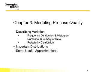
Chapter 3. Modeling Process Quality. Stem-and-Leaf Display. numbers above. numbers within. Percentile Sample median or fiftieth percentile First quartile (Q1), third quartile (Q3) Interquartile range (Q3-Q1). numbers below. Plot of Data in Time Order.

E N D
Stem-and-Leaf Display numbers above numbers within • Percentile • Sample median or fiftieth percentile • First quartile (Q1), third quartile (Q3) • Interquartile range (Q3-Q1) numbers below
Plot of Data in Time Order Marginal plot produced by MINITAB
Histograms – Useful for large data sets • Group values of the variable into bins, then count the number of observations that fall into each bin • Plot frequency (or relative frequency) versus the values of the variable
Numerical Summary of Data Samples: x1, x2, x3, … , xn Sample average: Previous wafer thickness example:
Sample Variance: Sample Standard Deviation: Previous wafer thickness example:
The Box Plot(or Box-and-Whisker Plot) Sample median Q3 Q1 maximum minimum Box plots can identify potential outliers.
Probability Distributions • Statistics: based on sample analysis involving measurements • Probability: based on mathematical description of abstract model • Random variable: (real) value associated with variable of interest • Probability distribution: probability of occurrence of variable
Sometimes called a probability mass function Sometimes called a probability density function
Mean Variance
N: population D: class of interest within population n: random samples chosen from N x: belongs to class of interest among random samples
Example: A lot containing 100 products. There are five defects. Choose 10 random samples. Find the probability that one or fewer defects are contained in the sample. N = 100 D = 5 n = 10 x ≤ 1
The random variable x is the number of successes out of n independentBernoulli trials with constant probability of success p on each trial.
As λ gets large, p(x) looks more symmetric, i.e., looks like binomial. Binomial is an approximation for limiting Poisson distribution. n→∞ and p →0 such that np = λ, binomial distribution approximates Poisson distribution with λ.
The random variable x is the number ofBernoulli trials upon which the rthsuccess occurs.
When r = 1 the Pascal distribution is known as the geometric distribution. • The geometric distribution has many useful applications in statistical quality control.
where and Φ(.) is a standard normal distribution with mean 0 and standard deviation 1.
Original normal distribution Standard normal distribution
Practical interpretation – the sum of independent random variables is approximately normally distributed regardless of the distribution of each individual random variable in the sum
When r is an integer, the gamma distribution is the result of summing r independently and identically exponential random variables each with parameter λ
When β = 1, the Weibull distribution reduces to the exponential distribution
Probability Plot • Determining if a sample of data might reasonably be assumed to come from a specific distribution • Probability plots are available for various distributions • Easy to construct with computer software (MINITAB) • Subjective interpretation
Other Probability Plots • What is a reasonable choice as a probability model for these data?
Approximations: H = hypergeometric, B = binomial, P = Poisson, N = normal