Download
1 / 16
160 likes | 262 Views
3-BC Working Points for 0.5 and 1.0 nC. tool/method – how to find working points (1D with CSR). example (1nC). example (0.5nC). some remarks. rf0a. rf0b. bc0. rf1. bc1. rf2. bc2. Tool / Method. E0. E1. E2. linear parameters:. e0’. e1’. e2’. q56_0. q56_1. q56_2.

E N D
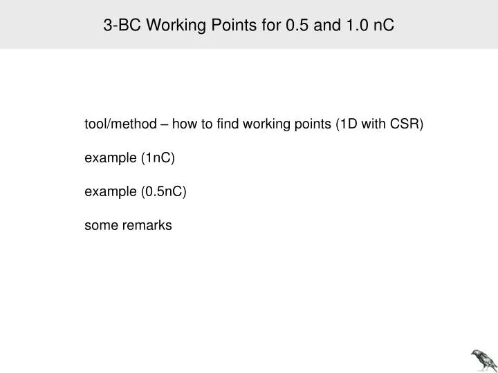
3-BC Working Points for 0.5 and 1.0 nC tool/method – how to find working points (1D with CSR) example (1nC) example (0.5nC) some remarks
rf0a rf0b bc0 rf1 bc1 rf2 bc2 Tool / Method E0 E1 E2 linear parameters: e0’ e1’ e2’ q56_0 q56_1 q56_2 non-linear param.: (knobs) e0’’ e0’’’ my definition:
rf0a rf0b bc0 rf1 bc1 rf2 bc2 Tool / Method E0 E1 E2 linear parameters: e0’ e1’ e2’ q56_0 q56_1 q56_2 C0 C1 2 Ctot non-linear param.: (knobs) e0’’ e0’’’
rf0a rf0b bc0 rf1 bc1 rf2 bc2 Tool / Method E0 E1 E2 in a b c d e out 1. track without self effects: in a,b,c,d,e,out in a,b,c,d,e,out (‘in’ with laser heater!) 2. track with SC&wakes: in a1 (Igor’s SC&wakes) re-adjust rf0 parameters: E0; rms{a1-a}=min in a2,b2,c1 re-adjust rf1 parameters: E1; rms{c1-c}=min in a2,b2,c2,d2,e1 re-adjust rf2 parameters: E2; rms{e1-e}=min in a2,b2,c2,d2,e2,out1 procedure takes about 1 min total compression not quite perfect <x1-x>≠0 … in principle: modify e2’ or q45_2 few iterations to adjust e0’’ and e0’’’
rf0a rf0b bc0 rf1 bc1 rf2 bc2 Tool / Method E0 E1 E2 in a b c d e out 3. track with …&…&CSR: in a1 re-adjust rf0 parameters: E0; rms{a1-a}=min in a2(1d-CSRtrack)b2,c1 re-adjust rf1 parameters: E1; rms{c1-c}=min in a2,b2,c2 (1d-CSRtrack) d2,e1 re-adjust rf2 parameters: E2; rms{e1-e}=min in a2,b2,c2,d2,e2 (1d-CSRtrack) out1 procedure takes about 30 min total compression not quite perfect few iterations to adjust e0’’ and e0’’’
(1d-CSRtrack) (matlab-controller) in = longitudinal phase space create lattice with design q56 csrtrk.in create artificial transverse phase space (n 1µm, initial , focus at last magnet) run CSRtrack {look for transverse properties} extract longitudinal phase space out
example (1nC) C0=1.80; C1=19.0/C0; C2=100.0/(C0*C1); q56_0=0.040; q56_1=0.110; q56_2=0.027764039; without self effects e0ss =0.0; e0sss=0.0; e0ss =0.5; e0sss=0.0; e0ss =1.0; e0sss=0.0;
example (1nC) C0=1.80; C1=19.0/C0; C2=100.0/(C0*C1); q56_0=0.040; q56_1=0.110; q56_2=0.027764039; without self effects e0ss =0.75; e0sss=0.0; e0ss =0.82; e0sss=0.0; e0ss =0.88; e0sss=0.0;
example (1nC) C0=1.80; C1=19.0/C0; C2=100.0/(C0*C1); q56_0=0.040; q56_1=0.110; q56_2=0.027764039; with wakes, without CSR e0ss =0.75; e0sss=0.0; e0ss =0.82; e0sss=0.0; e0ss =0.88; e0sss=0.0;
example (1nC) C0=1.80; C1=19.0/C0; C2=100.0/(C0*C1); q56_0=0.040; q56_1=0.110; q56_2=0.027764039; with wakes & CSR e0ss =0.68; e0sss=0.0; e0ss =0.75; e0sss=0.0; e0ss =0.82; e0sss=0.0;
example (1nC) C0=1.80; C1=19.0/C0; C2=100.0/(C0*C1); q56_0=0.040; q56_1=0.110; q56_2=0.027764039; with wakes & CSR e0ss =0.68; e0sss=-1.0; e0ss =0.68; e0sss=0.0; e0ss =0.68; e0sss=1.0;
example (1nC) C0=1.80; C1=19.0/C0; C2=100.0/(C0*C1); q56_0=0.040; q56_1=0.110; q56_2=0.027764039; with wakes & CSR e0ss =0.68; e0sss=0.0;
example (0.5nC) C0=1.80; C1=19.0/C0; C2=200.0/(C0*C1); q56_0=0.040; q56_1=0.110; q56_2=0.031020315; with wakes & CSR with wakes without CSR e0ss =0.85; e0sss=0.0; e0ss =0.85; e0sss=1.0; e0ss =0.78; e0sss=1.0;
some remarks its is easy to find working points (on the computer) slight rollover of tails same peak current with 0.5 nC: reduce effects before BC3 double BC3 compression tighter tolerances same LH power twice uncorrelated energy spread same energy spread increased µB-gain stronger CSR effects in BC3 (steady state, R ~ const, same peak current) effects after BC3 are not decreased / might be increased
1.0nC 0.5nC E is doubled x’ x’
140 120 100 80 60 40 1.5 2.0 2.5 3 VB VA q56 C E tol. V3.9 end-chirp noise /mm *100 *1000 MV MV@1 A VA 40 1.8 2.70.758 30.2 7.4 73 VB 60 1.8 1.8 0.57 30.9 7.4 125 VA-h 40 1.8 2.7 0.39 31 7.4 130 CB-h 60 1.8 1.8 0.313 32 7.5 190 0.5 nC working point same energy spread C_tot*E_LH