Download
1 / 62
630 likes | 718 Views
Intro. To GIS Lecture 10 Model Builder May 6 th , 2013. Reminders. Please turn in your homework The final lab is on Wednesday (5/8/2013).

E N D
Reminders • Please turn in your homework • The final lab is on Wednesday (5/8/2013). • For those of you interested, an optional (bonus) lab (Model builder + Spatial autocorrelation) will be assigned on Monday 13th . This is due on Monday 20th (final test).
REVIEW: How to represent the real world in 3D? • Data points are used to generate a continuous surface. In the below example, a color coded surface is generated from sample values
REVIEW: How to represent the real world in 3D? • Two ways to generate real world surfaces from point data (sample values) • Vector • raster • Whatever the method, what kind of data are available to represent the world?
REVIEW: Samples could represent any quantity (value) • Elevation • Climate data • Temperature • Precipitation • Wind • CO2 flux • Others • Ice thickness • Spatial samples (of some quantity) in a city • Gold concentrations • LiDAR data points
Vector representation (of surfaces) • Triangular Irregular Network (TIN) • TIN can be used to • Generate contour lines • Slope • Aspect
Triangular Irregular Network • Way of representing surfaces (vector) • Elevation points connected by lines to form triangles • Size of triangles may vary • Each face created by a triangle is called a facet
REVIEW: Delaunay triangulation Delaunay triangles: all satisfy the condition Delaunay NOT satisfied
Raster Representation (of surfaces) • The most commonly used term for raster representation is Digital Elevation Model (DEM) • Any digital model for any other variable could be generated • For DEM, each cell has an elevation (z-value) • To generate DEM from sample points, interpolation is used to fill in between surveyed elevations – several methods to choose from
REVIEW: Spatial Interpolation • Generating surface from points (samples) based upon: • Nearest Neighbor • Inverse Distance Weighted (IDW) • Kriging • Splining
REVIEW: Nearest-Neighbor • Uses elevations (or another quantity) from a specified number of nearby control points Sample with Known value Pixel (grid cell) with unknown value
REVIEW: Inverse Distance Weighted (IDW) • Spatial Autocorrelation • Near objects are more similar than far objects • IDW weights point values based on distance
REVIEW: Inverse Distance Weighted (IDW) • Estimating an unknown value for a pixel (p) by weighting the sample values based on their distance to (p) i=8 in this example j • In the above equation, n is the power. It is usually equals to 2, i.e., n=2. But you can pick n=1, n=1.5, etc.
REVIEW: IDW – Choosing the Power • Power setting influences interpolation results • Lower power results in smoother surfaces • Higher power results in rugged surface (it become more like ….?)
REVIEW: Kriging • Statistical regression method, whose process consists of two main components • Spatial autocorrelation (semivariance) • Some weighting scheme • Advanced interpolation function, can adapt to trends in elevation data
REVIEW: Krigingand Semivariogram • Semivarigram is a graph describing the semivariance (or simply variance) between pairs of samples at different distances (lags) • The idea comes from intuition: • Things that are spatially close are more correlated than those are far way (similar to IDW)
REVIEW: Generating Semivariogram • To generate a semivariogram, semivariance between pairs of points (for various distances/lags) are to be calculated
REVIEW: Krigingand Semivariogram • The first step in the kriging algorithm is to compute an average semivariogram for the entire dataset. This is done by going through each single point in the dataset and calculate semivariogram. Then the semivariogram are averaged. • The second step is to calculate the weights associated with each point
REVIEW: Spline Interpolation • Curves fit through control points • Interpolated values may exceed actual elevation values • Regularized vs. Tension options
Evaluation of the generated surface • Independent samples must be preserved for accuracy assessment of the predicted (generated) surface. These points are called check points. • In other words, if you have 100 samples in the area, you’d use 90 to create the surface and 10 of them to evaluate how accurately the surface represents the actual world
Evaluation • Using check points # of check points Prediction Observation
04_02_Figure Accuracy Vs. Precision
Model Builder • Credit • Rowan University
Geoprocessing • When we perform geoprocessing tasks on our data, we are developing the components of a GIS model. • We perform geoprocessing every time we: • Use a tool interactively in ArcMap • Use tools from ArcToolbox • Execute commands using the command line • Connect tools in ModelBuilder • Use functions in a script (like Python)
Static and Dynamic • Static modeling is the series of steps required to achieve some final result. • Available land for development of a nursery • Siting of cell towers • Dynamic modeling is performed in a similar fashion, but has additional parameters requiring several iterations of the model. • Disease outbreak modeling • Real-time traffic analysis • Spread of wildfires, heavy rain, etc.
Why Use ModelBuilder? • Developing a model for a GIS analysis allows for repeat testing of a hypothesis using different data. • The model can be coded into a GIS application, so that the steps are performed automatically. • Allows experimentation with model parameters – particularly for “weighting and rating” • Easier reproduction of results. • Simplification of workflow. • Informs the computer how to conduct a series of steps that would be impractical for you to do manually.
Why Use ModelBuilder? • An automation tool… • Common Types of Models • Spatial analysis • Example: suitability – building attractiveness maps
Reproducibility • In performing an analysis, you must have your workflow clearly defined. • This ensures that you are performing the steps in the correct order using the appropriate tools. • Missteps are easy, especially when there can be hours of computer processing between steps. • The GIS model can be exported as a graphic flowchart or a modeling data structure.
Workflow Efficiency • There are many repetitive steps you will take in your daily workflow. • Streamlining the process saves you time. • If you always start working in a File Geodatabase with specific resolution and projection information, a model for generating your specialized GDB can be created.
Human Inefficiency • You physically cannot perform the steps as fast as GIS can produce the results. • Certain steps, such as iteration through a feature set would be prohibitively time consuming. • You must perform the same steps 21 times to clip data to each individual NJ county. • Rail use analysis: 200+ stations • Minimize the amount of time spent “babysitting” GIS to perform complex analyses.
How do we model? • ArcGIS has a drag-and-drop interface to ArcToolbox called ModelBuilder allowing you to develop a flow chart of your GIS workflow. • This flowchart is then run step by step to perform your analysis. • ArcGIS allows for custom scripting that can be added to ArcToolbox, introducing greater functionality. • Custom export scripts, specialized versions of existing tools, develop tools not available in ArcToolbox.
Introduction to ModelBuilder • Over the past semester, we've performed several geoprocessing tasks • We have used geoprocessing tools in sequence to analyze GIS data • ArcGIS allows you to link tools together to create a workflow
How ModelBuilder Works • Drag layers you want to participate into the model • Drag tools you want to use into the model • Output layers, tables, objects shown in green • Connect the features using arrows • Order matters to certain tools (Clip)
Model Builder Elements • Project elements (blue ovals) exist prior to model • Tool to be executed (yellow rectangle) • Derived data (green ovals) produced by tool • Connector (arrow) showing sequence of processing • Value or variable (light blue oval)…such as numbers, strings, spatial references, and geographic extents. • Derived value (light green oval)