Download
1 / 18
180 likes | 287 Views
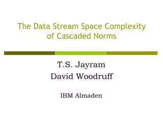
The Data Stream Space Complexity of Cascaded Norms. T.S. Jayram David Woodruff IBM Almaden. Data streams. Algorithms access data in a sequential fashion One pass / small space Need to be randomized and approximate [FM, MP, AMS]. Algorithm. Main Memory.

E N D
The Data Stream Space Complexity of Cascaded Norms T.S. Jayram David Woodruff IBM Almaden
Data streams • Algorithms access data in a sequential fashion • One pass / small space • Need to be randomized and approximate • [FM, MP, AMS] Algorithm Main Memory 2 3 4 16 0 100 5 4 501 200 401 2 3 6 0
Frequency Moments and Norms • Stream defines updates to a set of items 1,2,…,d. • fi= weight of item i • positive-only vs. turnstile model • k-th Frequency Moment Fk = i |fi|k • p-th Norm: Lp = kfkp= (i |fi|p)1/p • Maximum frequency: p=1 • Distinct Elements: p=0 • Heavy hitters • Assume length of stream and magnitude of updates is · poly(d)
Classical Results • Approximating Lp and Fp is the same problem • For 0 · p · 2, Fp is approximable in O~(1) space (AMS, FM, Indyk, …) • For p > 2, Fp is approximable in O~(d1-2/p) space (IW) • this is best-possible (BJKS, CKS)
Cascaded Aggregates • Stream defines updates to pairs of items in {1,2,…n} x {1,2,…,d} • fij = weight of item (i,j) • Two aggregates P and Q Q P P ± Q P ± Q = cascaded aggregate
Motivation • Multigraph streams for analyzing IP traffic [Cormode-Muthukrishnan] • Corresponds to P ± F0 for different P’s • F0 returns #destinations accessed by each source • Also introduced the more general problem of estimating P ± Q • Computing complex join estimates • Product metrics [Andoni-Indyk-Krauthgamer] • Stock volatility, computational geometry, operator norms
n 1 n1-2/k d1-2/p k=p n1-1/k n1-1/k n1-2/k d ? 2 1 d d1-2/p £(1) 0 £(1) p 0 1 2 1 The Picture We give the(n1-1/k) bound for Lk± L0 and Lk± L1 Õ(n1/2) for L2± L0 without deletions [CM] Õ(n1-1/k) for Lk± Lpfor any p in {0,1} in turnstile [MW] k Follows from techniques of [ADIW] [Ganguly] (without deletions) Our upper bound We give a 1-pass O~(n1-2/kd1-2/p) space algorithm when k ¸ p We also provide a matching lower bound based on multiparty disjointness Estimating Lk± Lp
Our Problem: Fk± Fp M = Fk± Fp (M) = i (j |fij|p)k = i Fp(Row i)k
High Level Ideas: Fk± Fp How do we do the sampling efficiently?? • We want the Fk-value of the vector (Fp(Row 1), …, Fp(Row n)) • We try to sample a row i with probability / Fp(Row i) • Spend an extra pass to compute Fp(Row i) • Could then output Fp(M) ¢ Fp(Row i)k-1 (can be seen as a generalization of [AMS])
Review – Estimating Fp [IW] • Level sets: • Level t is good if |St|(1+ε)2t¸ F2/B • Items from such level sets are also good
²-Histogram [IW] • Finds approximate sizes s’t of level sets • For all St, s’t· (1+ε)|St| • For good St, s’t¸ (1- ε)|St| • Also provides O~(1) random samples from each good St • Space: O~(B)
Sampling Rows According to Fp value • Treat n x d matrix M as a vector: • Run ε-Histogram on M for certain B • Obtain (1§ε)-approximation st’ to |St| for good t • Fk± Fp(M’) ¸ (1-ε) Fk± Fp(M), where M’ is M restricted to good items (Holder’s inequality) • To sample, • Choose a good t with probability st’(1+ε)pt/Fp’(M), where Fp’(M) = sumgood t st’ (1+ε)pt • Choose random sample (i, j) from St • Let row i be the current sample Pr[row i] = t [st’(1+ε)pt/Fp’(M)]¢[|StÅ row i|/|St|] ¼ Fp(row i)/Fp(M) Problems High level algorithm requires many samples (up to n1-1/k) from the St, but [IW] just gives O~(1). Can’t afford to repeat in low space 2. Algorithm may misclassify a pair (i,j) into St when it is in St-1
High Level Ideas: Fk± Fp • We want the Fk-value of the vector (Fp(Row 1), …, Fp(Row n)) • We try to sample a row i with probability / Fp(Row i) • Spend an extra pass to compute Fp(Row i) • Could then output Fp(M) ¢ Fp(Row i)k-1 (can be seen as a generalization of [AMS]) How do we avoid an extra pass??
Avoiding an Extra Pass • Now we can sample a Row i / Fp(Row i) • We design a new Fk-algorithm to run on (Fp(Row 1), …, Fp(Row n)) which only receives IDs i with probability/ Fp(Row i) • For each j 2 [log n], algorithm does: 1. Choose a random subset of n/2j rows 2. Sample a row i from this set with Pr[Row i] / Fp(Row i) • We show that O~(n1-1/k) oracle samples is enough to estimate Fk up to 1§ε
New Lower Bounds Alice Bob n x dmatrix B n x dmatrix A NO instance: for all rows i, ¢(Ai, Bi) · 1 YES instance: there is a unique row j for which ¢(Aj, Bj) = d, and for all i j, ¢(Ai, Bi) · 1 We show distinguishing these cases requires (n/d)randomized communication CC Implies estimating Lk(L0) or Lk(L1) needs (n1-1/k) space
Information Complexity Paradigm • [CSWY, BJKS]: the information cost IC is the amount of information the transcript reveals about the inputs • For any function f, CC(f) ¸ IC(f) • Using their direct sum theorem, it suffices to show an (1/d) information cost of a protocol for deciding if¢(x,y) = dor¢(x,y) · 1 • Caveat: distribution is only on instances where ¢(x,y) · 1
d a e f c b Working with Hellinger Distance • Given the prob. distribution vector ¼(x,y) over transcripts of an input (x,y) • Let Ã(x,y)¿ = ¼(x,y)¿1/2 for all ¿ • Information cost can be lower bounded by E¢(u,v) = 1 kÃ(u,u) - Ã(u,v)k2 • Unlike previous work, we exploit the geometry of the squared Euclidean norm (useful in later work [AJP]) • Short diagonals property: E¢(u,v) = 1 kÃ(u,u) - Ã(u,v)k2 ¸(1/d)E¢(u,v) = d kÃ(u,u) - Ã(u,v)k2 a2 + b2 + c2 + d2 ¸ e2 + f2
Open Problems • Lk± Lpestimation for k < p • Other cascaded aggregates, e.g. entropy • Cascaded aggregates with 3 or more stages