Download
1 / 23
230 likes | 369 Views
ACADEMY OF ECONOMIC STUDIES DOCTORAL SCHOOL OF FINANCE AND BANKING. COMMON VOLATILITY TRENDS AMONG CENTRAL AND EASTERN EUROPEAN CURRENCIES. MSc Student: ODANGIU ANDREEA RALUCA Coordinator: Professor MOISĂ ALTĂR. Bucharest, July 2007. Dissertation paper outline.

E N D
ACADEMY OF ECONOMIC STUDIES DOCTORAL SCHOOL OF FINANCE AND BANKING COMMON VOLATILITY TRENDS AMONG CENTRAL AND EASTERN EUROPEAN CURRENCIES MSc Student: ODANGIU ANDREEA RALUCA Coordinator: Professor MOISĂ ALTĂR Bucharest, July 2007
Dissertation paper outline • The importance of common trends in CEE exchange rate volatility • The aims of the present paper • Brief review of recent literature on exchange rate volatility • The data • The Component GARCH model • The Spillover Index • The Orthogonal GARCH model • Concluding remarks • References
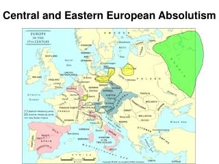
The importance of common trends in CEE exchange rate volatility • For the 12 new member states of the EU, adopting the euro as the national currency some time in the next few years is not optional; it is a definite requirement • Before adopting the euro, every country has to be part of ERM II, for at least two years • We examine the exchange rate volatility patterns of the Czech Republic, Hungary, Poland, Romania and Slovakia, over the sample period May 2001 – April 2007 • Poland is the only one of the twelve new member states that has not yet proposed a definite deadline for euro adoption, while Slovakia has already joined ERM II as of 28 November 2005. However, due to constant appreciation pressures on the koruna, the Slovak Central Bank has had to intervene frequently on the foreign exchange market, and eventually gain approval from the European Central Bank to lift the central parity rate by 8.5% as of 19 March 2007. The RON also faces similar appreciation pressures, which is one of the reasons why the National Bank of Romania has cut its monetary policy rate four times already since the beginning of 2007. Hungary was forced to postpone its plan to adopt the euro in 2010 after running up the European Union’s widest budget deficit in 2006.
The aims of the paper • To identify a unitary model for the five exchange rate volatilities and to identify similar patterns among them; • To isolate the different sources of exchange rate volatility and to compute a measure for how much the currencies influence each other; • To examine how the correlations between these five currencies have evolved over the time period under analysis.
Brief literature review • Teräsvirta (2006): extensive review of several univariate GARCH models • The Component GARCH model: introduced by Engle and Lee (1993), used in recent papers such as Maheu (2005), Guo and Neely (2006), Christoffersen et al. (2006) and Bauwens and Storti (2007) • Exchange rate volatility: Byrne and Davis (2003) – G7 countries; Kóbor and Székely (2004), Pramor and Tamirisa (2006)– CEE currencies; Borghijs and Kuijs (2004)- SVAR approach to examine the usefulness of flexible exchange rates as shock absorbers in CEE countries • Spillover Index: Diebold and Yilmaz (2007) • Orthogonal GARCH model: Klaassen (1999), Alexander (2000)
The Data • Daily nominal exchange rates of five CEE currencies against the euro, namely the Czech koruna (CZK), the Hungarian forint (HUF), the Polish zloty (PLN), the Romanian new leu (RON) and the Slovak koruna (SKK). The data is obtained from Eurostat (for SKK) and from the web site of each Central Bank respectively (for CZK, HUF, PLN and RON). Each exchange rate is quoted as number of national currency units per euro • The sampling period covers 4 May 2001 to 5 April 2007; we will also be studying two sub-periods, May 2001 to November 2004 and December 2004 to April 2007 • All series in levels display a unit root, as evident from the ADF test results. Hence the series are transformed into log-differences and we obtain the continuously compounded exchange rate returns (which are I(0)):
The Component GARCH Model The conditional variance in the GARCH(1,1) model can be written as: Allowing for the possibility that σ2 is not constant over time, but a time-varying trend qt, yields: where Dt is a slope dummy variable that takes the value Dt = 1 for εt < 0 and Dt = 0 otherwise, in order to capture any asymmetric responses of volatility to shocks. We test for the significance of this term using the Engle-Ng test for sign bias and include it where relevant. qt is the permanent component (or trend) of the conditional variance, while ht-qt is the transitory component. Stationarity of the CGARCH model and non-negativity of the conditional variance are ensured if the following inequality constraints are satisfied: 1 > ρ > (α+β), β > Φ > 0, α > 0, β > 0, Φ > 0, ω > 0.
Ljung-Box Test m=15 lags The results show a tremendous improvement in the values of the Q* statistics over the ones for the squared returns, so the component model successfully captures the typical pattern of serial correlation. All the Engle-Ng tests, Ljung-Box tests and CGARCH estimates have been computed using Rats 6.01.
Remarks • The autoregressive parameters in the trend equations, ρ, is very close to one for all currencies and all time periods (the smallest being 0.9467 for RON 2004 – 2007), so the series are very close to being integrated. • The shock effects on the transitory component of volatilities (the α coefficients), are much larger than the shock effects on the permanent component (the φ coefficients) – generally around three to six times larger. However, as found in all the papers that use the CGARCH specification, the shocks to short-run volatility are very short-lived, even if they are stronger. • ρ and β coefficients are generally higher in the late sample period, while φ and α coefficients are smaller, which implies that volatility is becoming less responsive to shocks and more persistent. The only exception is the RON. • The asymmetric effects are highly significant for HUF and PLN (for all sample periods). γcoefficients are consistently negative, which indicates that negative returns actually decrease variances, and that exchange rate volatility is lower during times of currency appreciation. • The five currencies appear to respond to temporary market shocks in similar ways (as suggested by positive correlations between transitory volatilities), they respond differently to more permanent shocks.
The Spillover Index The typical representation of a covariance stationary first-order VAR is: The optimal 1-step-ahead forecast is: and the corresponding 1-step-ahead error vector (assuming a two-variable VAR): where ut = Qtεt, and Qt-1 is the unique lower-triangular Cholesky factor of the covariance matrix of εt. For the pth-order N-variable VAR using H-step-ahead forecasts, the Spillover Index is:
Remarks • The appropriate number of lags for each VAR model is determined using the information criteria. We also perform a check on the AR roots, and the results indicate that all six VAR specifications are stable. • We use 20-step-ahead forecast error variance and a Cholesky ordering as shown in the table headers. The reasons behind these decisions are as follows: volatility has been found to be highly persistent (especially the trend component), so a large enough number of forecast steps is necessary; furthermore, according to Brooks (2002), the differences between the different Cholesky orderings become smaller as the number of forecast periods increases. • The results clearly indicate that volatility spillovers have increased over time, in line with the findings of Kóbor and Székely (2004) but contrary to Pramor and Tamirisa (2006). Furthermore, spillovers into permanent volatility appear stronger than into the transitory component. • While the results are sensitive to series ordering, in many cases the HUF appears to have been the most important source of volatility in the region, while the PLN has been the most important shock absorber. Pramor and Tamirisa (2006) and Borghijs and Kuijs (2004) reach similar conclusions.
The Orthogonal GARCH Model The steps involved in estimating this model are as follows: Step 1: Computing the principal components of the normalized initial system: Step 2: Estimating the conditional variance of the principal components by standard univariate GARCH(1,1) models: for every principal component j, l = 1,…,k (j ≠ l). Step 3: Transform the conditional moment of the principal components into the ones for the original series: where A = (ω*ij) = wijσi
The Orthogonal GARCH Model • We follow the approach of Klaassen (1999) and we consider the same number of principal components as series in the initial system. This presents several advantages, such as eliminating the problem of the arbitrary choice of k or avoiding the danger of losing important information about the initial system by ignoring the last components, which may sometimes contain more than just ‘noise’. • The most influential component is the first one, but it only explains just over 40%. This is to be expected, because the correlations between the original series are not very high to begin with (at least when compared to industrial countries). • The fifth component accounts for almost 10%, which is quite high.
Evolution of 3 Selected Conditional Correlations, With 60-day Moving Averages Higher volatility is generally associated with higher correlation coefficients among the CEE currencies. Examination of the longer-term trends of correlations reveals that they have generally increased over the sample period in question (May 2001 – April 2007), or at least remained at broadly similar levels. The only exception: CZK - SKK
Concluding Remarks • Many papers have focused on the degree of business cycle convergence; however, we believe that exchange rate volatility is also a very important aspect, especially when entering ERM II, prior to actual changeover. Under these circumstances, an analysis such as ours is important because it appears essential for Central Banks to know very well the exchange rate volatility patterns of their country’s own currency, but also the ones of the other currencies in the region, in order to have better expectations of how the exchange rate is going to be affected. • We find evidence of higher correlations of volatility components, increasing spillovers and higher conditional correlations among currencies, which suggest growing convergence and stronger cross-linkages between the five exchange rates in question. • Policy makers of each country have to increasingly take into account other countries’ actions when making their own decisions. This calls for more coordinated courses of action, which would be a very good exercise in preparation for euro adoption and a single, unified monetary policy. • Possible directions for future research: estimate volatilities with more complex models, such as smooth transition or Markov-switching GARCH, or using intra-day returns; a study of contagion phenomena among the CEE currencies, especially during turbulent market times, using one of the approaches presented in Dungey et al. (2004).
References • Alexander, C. (2000), “Orthogonal Methods for Generating Large Positive Semi-Definite Covariance Matrices”, Discussion Papers in Finance 2000-06, ICMA Centre, The University of Reading • Alexander, C. (2001), “Market Models. A Guide to Financial Analysis”, John Wiley & Sons Ltd. • Andersen, T.G., Bollerslev, T., Christoffersen, P.F. and Diebold, F.X. (2005), “Practical Volatility and Correlation Modelling for Financial Market Risk Management”, NBER Working Paper 11069 • Andersen, T.G., Bollerslev, T., Diebold, F.X. and Labys, P. (2000), “Exchange Rate Returns Standardized by Realized Volatility are (Nearly) Gaussian”, NBER Working Paper 7488 • Bauwens, L. and Storti, G. (2007), “A Component Garch Model With Time Varying Weights”, CORE Discussion Paper 2007/19 • Borghijs, A. and Kuijs, L. (2004), “Exchange Rates in Central Europe: A Blessing or a Curse?”, IMF Working Paper 04/2 • Brooks, C. (2002), “Introductory Econometrics for Finance”, Cambridge University Press • Bufton, G. and Chaudhri, S. (2005), “Independent Component Analysis”, Quantitative Research, Royal Bank of Scotland • Byrne, J.P. and Davis, P.E. (2003), “Panel Estimation Of The Impact Of Exchange Rate Uncertainty On Investment In The Major Industrial Countries”, NIESR Working Paper • Christoffersen, P.F., Jacobs, K. and Wang, Y. (2006), “Option Valuation with Long-run and Short-run Volatility Components”, Working Paper, McGill University • Diebold, F.X. and Yilmaz, K. (2007), “Measuring Financial Asset Return and Volatility Spillovers, With Application to Global Equity Markets”, Manuscript, Department of Economics, University of Pennsylvania • Dungey, M., Fry, R. Gonzales-Hermosillo, B. and Martin, V. (2004), “Empirical Modeling of Contagion: A Review of Methodologies”, IMF Working Paper 04/78
References • Égert, B. and Morales-Zumaquero, A. (2005), “Exchange Rate Regimes, Foreign Exchange Volatility and Export Performance in Central and Eastern Europe: Just Another Blur Project?”, BOFIT Discussion Papers 8/2005 • Engle, R.F. and Lee, G.G.J. (1993), “A Permanent and Transitory Component Model of Stock Return Volatility”, Discussion Paper 92-44R, University of California, San Diego • Fidrmuc, J. and Korhonen, I. (2004), “A meta-analysis of business cycle correlation between the euro area and CEECs: What do we know – and who cares?”, BOFIT Discussion Papers 2004 No. 20 • Guo, H. and Neely, C. (2006), “Investigating the Intertemporal Risk-Return Relation in International Stock Markets with the Component GARCH Model”, Working Paper 2006-006A, Federal Reserve Bank of St. Louis • Klaassen, F. (1999), “Have Exchange Rates Become More Closely Tied? Evidence from a New Multivariate GARCH Model”, Discussion Paper 10/1999, CentER and Department of Econometrics, Tilburg University • Kóbor, Á. and Székely, I.P. (2004), “Foreign Exchange Market Volatility in EU Accession Countries in the Run-Up to Euro Adoption: Weathering Uncharted Waters”, IMF Working Paper 04/16 • Maheu, J. (2005), “Can GARCH Models Capture Long-Range Dependence?”, Studies in Nonlinear Dynamics & Econometrics, Volume 9, Issue 4, Article 1 • Pramor, M. and Tamirisa, N.T. (2006), “Common Volatility Trends in the Central and Eastern European Currencies and the Euro”, IMF Working Paper 06/206 • Teräsvirta, T. (2006), “An Introduction to Univariate GARCH Models”, SSE/EFI Working Papers in Economics and Finance, No. 646, Stockholm School of Economics • *** European Central Bank, Convergence Report May 2006