Download
1 / 58
580 likes | 583 Views
Learn how to find and control active constraints, optimize variables, manipulate throughput, select stabilizing control variables, and design a supervisory layer in plantwide control systems. Explore case studies in distillation and understand the dos and don'ts of distillation column control.

E N D
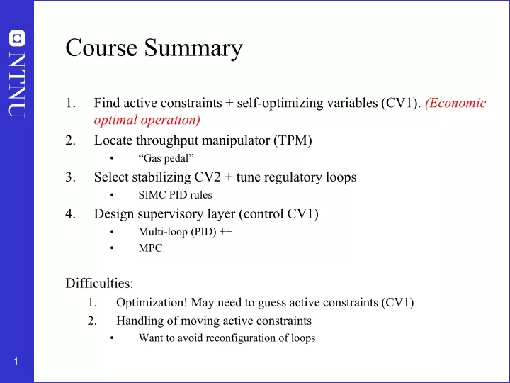
Course Summary • Find active constraints + self-optimizing variables (CV1). (Economic optimal operation) • Locate throughput manipulator (TPM) • “Gas pedal” • Select stabilizing CV2 + tune regulatory loops • SIMC PID rules • Design supervisory layer (control CV1) • Multi-loop (PID) ++ • MPC Difficulties: • Optimization! May need to guess active constraints (CV1) • Handling of moving active constraints • Want to avoid reconfiguration of loops
Summary: Sigurd’s plantwide control rules Rules for CV1-selection: 1. Control active constraints • Purity constraint on expensive product is always active (overpurification gives loss): 2. Unconstrained degrees of freedom (if any): Control “self-optimizing” variables (c). • The ideal variable is the gradient of J with respect to the inputs (Ju = dJ/du), which always should be zero, independent of disturbances d, but this variable is rarely available • Exception (if available!): Parallel systems (stream split, multiple feed streams/manifold) with given throughput (or given total gas flow, etc.) • Should have equal marginal costs Jiu = dJi/du, so Ju = J1u - J2u, etc. • Heat exchanger splits: equal Jächke temperatures, JT1 = (T1 – Th1)^2/(T1-T0) • In practice, one prefers to control single variables, c=Hy (where y are all available measurements and H is a selection matrix), which are easy to measure and control, and which have the following properties: • Optimal value for c is almost constant (independent of disturbances): Want small magnitude of dcopt(d)/dd. • Variable c is sensitive to changes in input: Want large magnitude of gain=dc/du (this is to reduce effect of measurement error and noise). • If the economic loss with single variables is too large, then one may use measurement combinations, c=Hy (where H is a “full” matrix). 3. Unconstrained degrees of freedom: NEVER try to control a variable that reaches max or min at the optimum (in particular, never control J) • Surprisingly, this is a very common mistake, even (especially?) with control experts Ruke for TPM location: Locate TPM at thenextconstraint to becomeactive as throughput is increased (bottleneck) Rules for inventory control: 1. Use Radiation rule (PC, LC, FC ++) 2. Avoid having all flows in a recycle system on inventory control (this is a restatement of Luyben’s rule of “fixing a flow inside a recycle system” to avoid snowballing) Rules for selecting stabilizing CVs (CV2): Control sensitive variablkes Rules for pairing: 1. General: “Pair close” (large gain and small effective time delay) 2. CV1: Sigurd’s pairing rule: “Pair MV that may (optimally) saturate with CV that may be given up” 3. CV2 (stabilizing loop): Avoid MV that may saturate
PLANTWIDE CONTROLCASE STUDIES • Distillation: regulatory control • Distillation: Economics (CV1) • Single column • Two columns in series • Reactor/separator/recycle problem • Economics (CV1) • TPM location • Max. throughput (Bottleneck)
Case study: Distillation control • S. Skogestad, ``The dos and don'ts of distillation columns control'', Chemical Engineering Research and Design (Trans IChemE, Part A), 85 (A1), 13-23 (2007).
Typical “LV”-regulatory control Assume given feed 5 dynamic DOFs (L,V,D,B,VT) Overall objective (CV1): Control compositions (xD and xB) “Obvious” stabilizing loops (CV2): • Condenser level (M1) • Reboiler level (M2) • Pressure (p) + “non-obvious” CV2 4. Column temperature (T)
L Ts TC TC V Issues distillation control • The “configuration” problem (level and pressure control) • Which are the two remaining degrees of freedom? • e.g. LV-, DV-, DB- and L/D V/B-configurations • The temperature control problem • Which temperature (if any) should be controlled? • Composition control problem • Control two, one or no compositions? • Always control valuable product at spec
Configurations Control “configurations” (pairing u2-y2 for level control) • “XY-configuration” X: remaining input in top after controlling top level (MD): X= L (reflux), D, L/D,… Y: remaining input in bottom after controlling MB: Y = V (boilup, energy input), B, V/B, ...
Configurations LC Top of Column cooling VT LS “Standard” : LY-configuration (“energy balance”) L+D D L Set manually or from upper-layer controller (temperature or composition) Set manually or from upper-layer controller VT DS LC “Reversed”: DY-configuration (“material balance”) D L
Configurations Top of Column VT LC D L D Ls Set manually or from upper-layer controller (L/D)s x Similar in bottom... XV, XB, X V/B
Configurations How do the configurations differ? • Has been a lot of discussion in the literature (Shinskey, Buckley, Skogestad, Luyben, etc.). • Probably over-emphasized, but let us look at it • Level control by itself (emphasized by Buckley et al., 1985) • Interaction of level control with composition control • Related to “local consistency” (Do not want inventory control to depend on composition loops being closed) • “Self-regulation” in terms of disturbance rejection (emphasized by Skogestad and Morari, 1987) • Remaining two-point composition control problem (steady-state RGA - emphasized by Shinskey, 1984)
LV-configuration (most common) “LV-configuration”: • D and B for levels (“local consistent”) • L and V remain as degrees of freedom after level loops are closed Other possibilities: DB, L/D V/B, etc….
BUT: To avoid strong sensitivity to disturbances: Temperature profile must also be “stabilized” D feedback using e.g. D,L,V or B LIGHT TC F HEAVY B Even with the level and pressure loops closed the column is practically unstable - either close to integrating or even truly unstable ( e.g. with mass reflux: Jacobsen and Skogestad, 1991) • To stabilize the column we must use feedback (feedforward will give drift) • Simplest: “Profile feedback” using sensitive temperature
Stabilizing the column profile • Should close one “fast” loop (usually temperature) in order to “stabilize” the column profile • Makes column behave more linearly • Strongly reduces disturbance sensitivity • Keeps disturbances within column • Reduces the need for level control • Makes it possible to have good dual composition control • P-control usually OK (no integral action) • Similar to control of liquid level
Regulatory layer Stabilizing the column profile (T) . loop LV LV LV T T T s s s TC TC TC (a) Common: Control T using V (b) If V may saturate: Use L • T at which end? Prefer “important” end with tightest purity spec, • T at which stage? Choose “sensitive” stage (sensitive to MV change) • Pair T with which input (MV)? Generally “pair close” • But avoid input that may saturate • Dynamics: V has immediate effect, whereas L has delay • Prefer “same end” (L for Ttop, V for Tbtm) to reduce interactions • Note: may not be possible to satisfy all these rules TC TC TS
TC Bonus 1 of temp. control: Indirect level control Disturbance in V, qF: Detected by TC and counteracted by L -> Smaller changes in D required to keep Md constant!
Bonus 2 of temp. control: Less interactive Setpoint T: New “handle” instead of L Ts TC
Less interactive: Closed-loop response with decentralized PID-composition control Interactions much smaller with “stabilizing” temperature loop closed … and also disturbance sensitivity is expected smaller %
Integral action in inner temperature loop has little effect %
Note: No need to close two inner temperature loops % Would be even better with V/F
Would be even better with V/F: Ts TC F (V/F)s x V
x (L/F)s Ts TC A “winner”: L/F-T-conguration Only caution: V should not saturate
TC Temperature control: Which stage?
Binary distillation: Steady-state gain G0 = ΔT/ΔL for small change in L T / L BTM TOP
Summary: Which temperature to control? • Rule 1. Avoid temperatures close to column ends (especially at end where impurity is small) • Rule 2. Control temperature at important end (expensive product) • Rule 3. To achieve indirect composition control: Control temperature where the steady-state sensitivity is large (“maximum gain rule”). • Rule 4. For dynamic reasons, control temperature where the temperature change is large (avoid “flat” temperature profile). (Binary column: same as Rule 3) • Rule 5. Use an input (flow) in the same end as the temperature sensor. • Rule 6. Avoid using an input (flow) that may saturate.
Ls Ts TC Conclusion stabilizing control:Remaining supervisory control problem Would be even better with L/F With V for T-control + may adjust setpoints for p, M1 and M2 (MPC)
Summary step 5: Rules for selecting y2 (and u2) Selection of y2 • Control of y2 “stabilizes” the plant • The (scaled) gain for y2 should be large • Measurement of y2 should be simple and reliable • For example, temperature or pressure • y2 should have good controllability • small effective delay • favorable dynamics for control • y2 should be located “close” to a manipulated input (u2) Selection of u2 (to be paired with y2): • Avoid using inputs u2 that may saturate (at steady state) • When u2 saturates we loose control of the associated y2. • “Pair close”! • The effective delay from u2 to y2 should be small
Example (TPM location): Evaporator(with liquid feed, liquid heat medium, vapor product) PROBLEM: • Objective: “Keep p=ps (or T=Ts) if possible, but main priority is to evaporate a given feed” • CVs in order of priority: • CV1 = level, CV2 = throughput, CV3 = p • MV1 = feed pump, MV2 = heat fluid valve, MV3= vapor product valve • Constraints on MVs (in order of becoming active as throughput is increased): • Max heat (MV2), Fully open product valve (MV3), Max pump speed (MV1) • Where locate TPM? Pairings? Present structure has feed pump as TPM: May risk “overfeeding”
Pairing based on Sigurd’s general pairing rule**: • CV1=level with MV1 (top-priority CV is paired with MV that is least likely to saturate) • CV2=throughput with MV3 (so TPM =gas product valve) • CV3=p with MV2 (MV2 may saturate and p may be given up) • Note: Fully open gas product valve (MV3) is also the bottleneck • Rules agree because bottleneck is last constraints to become active as we increase throughput * General: Do not need a FC on the TPM **Sigurd’s general pairing rule: “Pair MV that may (optimally) saturate with CV that may be given up”
CASE STUDY: Recycle plant(Luyben, Yu, etc.)Part 1 -3 Recycle of unreacted A (+ some B) 5 Feed of A 4 1 2 Assume constant reactor temperature. Given feedrate F0 and column pressure: 3 Dynamic DOFs: Nm = 5 Column levels: N0y = 2 Steady-state DOFs: N0 = 5 - 2 = 3 Product (98.5% B)
Part 1: Economics (Given feed) Recycle plant: Optimal operation mT 1 remaining unconstrained degree of freedom, CV=?
J=V as a function of reflux L Optimum = Nominal point With fixed active constraints: Mr = 2800 kmol (max), xB= 1.5% A (max)
Control of recycle plant:Conventional structure (“Two-point”: CV=xD) LC TPM LC xD XC XC xB LC Control active constraints (Mr=max and xB=0.015) + xD
Luyben law no. 1 (to avoid snowballing): “Fix a stream in the recycle loop” (CV=F or D)
Luyben rule: CV=D (constant) LC LC XC LC
“Brute force” loss evaluation:Disturbance in F0 Luyben rule: Conventional Loss with nominally optimal setpoints for Mr, xB and c
Loss evaluation: Implementation error Luyben rule: Loss with nominally optimal setpoints for Mr, xB and c
Conclusion: Control of recycle plant Active constraint Mr = Mrmax Self-optimizing L/F constant: Easier than “two-point” control Assumption: Minimize energy (V) Active constraint xB = xBmin
Modified Luyben’s law to avoid snowballing • Luyben law no. 1 (“Plantwide process control”, 1998, pp. 57): “A stream somewhere in all recycle loops must be flow controlled” • Luybenruleis OK dynamically (short time scale), • BUT economically (steady-state): Recycle should increase with throughput • Modified Luyben’s law 1 (by Sigurd): “It must be a TPM or flow controlled on an intermediate time scale”
Part 2: TPM location Example Reactor-recycle process:Given feedrate (production rate set at inlet) TPM
Part 2: TPM location PC D L F0 F TC V B Note: Temperature and pressure controllers shown; Otherwise as before
TPM Alt.1 Alt.2 TPM TPM Alt.3 More? Alt. 5? Alt.6? Alt. 7? Alt.4 TPM=xAr TPM
T fixed in reactor Alt.1 Alt.2 Follows Luyben law 1: TPM inside recycle Alt.4 Alt.3 More? Alt. 5? Alt.6? Alt. 7? Not really comparable since T is not fixed Unconventional TPM
PC Alt. 5 What about TPM=D (Luyben rule)? • Control xB, xD, Md • Not so simple with liquid feed….. TPM LC LC ? XC TC LC XC
PC Alt. 5 What about TPM=D (Luyben rule)? Another alternative: • Top level control by boilup • Get extra DOF in top • OK! TPM LC LC XC TC LC XC
PC NOTE: There are actually two recycles • One through the reactor (D or F) • One through the column (L) • One flow inside both recycle loops: V • Alt.6: TPM=V if we want to break both recycle loops! TC
PC Alt. 6 TPM = V LC LC L XC TC F TPM XC LC Simulations (to be done) confirm This is the best! L and F for composition control: OK!
PC Alt. 7 What about keeping V constant?(in addition to having another TPM) LC TPM L LC TC F0 F V XC LC With feedrate F0 fixed (TPM) L for compostioncontrol in bottom (xB) Topcompositionfloating NO! Never control cost J=V
Reactor-recycle process: Want to maximize feedrate: reach bottleneck in column Bottleneck: max. vapor rate in column TPM