Download
1 / 7
70 likes | 76 Views
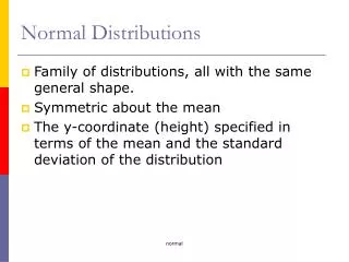
Normal Distributions. Normal Distributions One particularly important class of density curves are the Normal curves , which describe Normal distributions . All Normal curves are symmetric, single-peaked, and bell-shaped

E N D
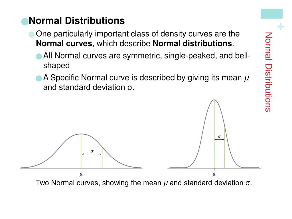
Normal Distributions • Normal Distributions • One particularly important class of density curves are the Normal curves, which describe Normal distributions. • All Normal curves are symmetric, single-peaked, and bell-shaped • A Specific Normal curve is described by giving its mean µ and standard deviation σ. Two Normal curves, showing the mean µ and standard deviation σ.
Normal Distributions • Normal Distributions • Definition: • A Normal distribution is described by a Normal density curve. Any particular Normal distribution is completely specified by two numbers: its mean µ and standard deviation σ. • The mean of a Normal distribution is the center of the symmetric Normal curve. • The standard deviation is the distance from the center to the change-of-curvature points on either side. • We abbreviate the Normal distribution with mean µ and standard deviation σ as N(µ,σ). Normal distributions are good descriptions for some distributions of real data. Normal distributions are good approximations of the results of many kinds of chance outcomes. Many statistical inference procedures are based on Normal distributions.
The 68-95-99.7 Rule Normal Distributions Although there are many Normal curves, they all have properties in common. • Definition:The 68-95-99.7 Rule (“The Empirical Rule”) • In the Normal distribution with mean µ and standard deviation σ: • Approximately 68% of the observations fall within σ of µ. • Approximately 95% of the observations fall within 2σ of µ. • Approximately 99.7% of the observations fall within 3σ of µ.
Example, p. 113 Normal Distributions The distribution of Iowa Test of Basic Skills (ITBS) vocabulary scores for 7th grade students in Gary, Indiana, is close to Normal. Suppose the distribution is N(6.84, 1.55). • Sketch the Normal density curve for this distribution. • What percent of ITBS vocabulary scores are less than 3.74? • What percent of the scores are between 5.29 and 9.94?
Normal Distributions • The Standard Normal Distribution • All Normal distributions are the same if we measure in units of size σ from the mean µ as center. Definition: The standard Normal distribution is the Normal distribution with mean 0 and standard deviation 1. If a variable x has any Normal distribution N(µ,σ) with mean µ and standard deviation σ, then the standardized variable has the standard Normal distribution, N(0,1).
Normal Distributions • The Standard Normal Table Because all Normal distributions are the same when we standardize, we can find areas under any Normal curve from a single table. • Definition:The Standard Normal Table • Table A is a table of areas under the standard Normal curve. The table entry for each value z is the area under the curve to the left of z. Suppose we want to find the proportion of observations from the standard Normal distribution that are less than 0.81. We can use Table A: P(z < 0.81) = .7910
Example, p. 117 Normal Distributions • Finding Areas Under the Standard Normal Curve Find the proportion of observations from the standard Normal distribution that are between -1.25 and 0.81. Can you find the same proportion using a different approach? 1 - (0.1056+0.2090) = 1 – 0.3146 = 0.6854