Download

1 / 10
100 likes | 103 Views
MDPs and the RL Problem. CMSC 471 – Spring 2014 Class #25 – Thursday, May 1 Russell & Norvig Chapter 21.1-21.3 Thanks to Rich Sutton and Andy Barto for the use of their slides (modified with additional slides and in-class exercise). Learning Without a Model.

E N D
MDPs and the RL Problem CMSC 471 – Spring 2014Class #25 – Thursday, May 1 Russell & Norvig Chapter 21.1-21.3Thanks to Rich Sutton and Andy Barto for the use of their slides(modified with additional slides and in-class exercise) R. S. Sutton and A. G. Barto: Reinforcement Learning: An Introduction
Learning Without a Model • Last time, we saw how to learn a value function and/or a policy from a transition model • What if we don’t have a transition model?? • Idea #1: • Explore the environment for a long time • Record all transitions • Learn the transition model • Apply value iteration/policy iteration • Slow and requires a lot of exploration! No intermediate learning! • Idea #2: Learn a value function (or policy) directly from interactions with the environment, while exploring R. S. Sutton and A. G. Barto: Reinforcement Learning: An Introduction
T T T T T T T T T T T T T T T T T T T T Simple Monte Carlo R. S. Sutton and A. G. Barto: Reinforcement Learning: An Introduction
TD Prediction Policy Evaluation (the prediction problem): for a given policy p, compute the state-value function Recall: target: the actual return after time t target: an estimate of the return γ: a discount factor in [0,1] (relative value of future rewards) R. S. Sutton and A. G. Barto: Reinforcement Learning: An Introduction
T T T T T T T T T T T T T T T T T T T T Simplest TD Method R. S. Sutton and A. G. Barto: Reinforcement Learning: An Introduction
Temporal Difference Learning • TD-learning: • Uπ (s) = Uπ (s) + α (R(s) + γ Uπ (s’) – Uπ (s))or equivalently:Uπ (s) = α [ R(s) + γ Uπ (s’) ] + (1-α) [ Uπ (s) ] • General idea: Iteratively update utility values, assuming that current utility values for other (local) states are correct Previous utility estimate Discount rate Learning rate Observed reward Previous utility estimate for successor state R. S. Sutton and A. G. Barto: Reinforcement Learning: An Introduction
Exploration vs. Exploitation • Problem with naive reinforcement learning: • What action to take? • Best apparent action, based on learning to date • Greedy strategy • Often prematurely converges to a suboptimal policy! • Random action • Will cover entire state space • Very expensive and slow to learn! • When to stop being random? • Balance exploration (try random actions) with exploitation (use best action so far) R. S. Sutton and A. G. Barto: Reinforcement Learning: An Introduction
Q-Learning Q-value: Value of taking action A in state S (as opposed to V = value of state S) R. S. Sutton and A. G. Barto: Reinforcement Learning: An Introduction
Q-Learning Exercise • Starting state: A • Reward function: in A yields -1 (at time t+1!); in B yields +1; all other actions yield -.1; G is a terminal state • Action sequence: • All Q-values are initialized to zero (including Q(G, *)) • Fill in the following table for the six Q-learning updates: A B G Q-learning reminder: R. S. Sutton and A. G. Barto: Reinforcement Learning: An Introduction
Q-Learning Exercise • Starting state: A • Reward function: in A yields -1 (at time t+1!); in B yields +1; all other actions yield -.1; G is a terminal state • Action sequence: • All Q-values are initialized to zero (including Q(G, *)); α and γ are 0.9 • Fill in the following table for the six Q-learning updates: A B G Q-learning reminder: R. S. Sutton and A. G. Barto: Reinforcement Learning: An Introduction