Download
1 / 50
500 likes | 623 Views
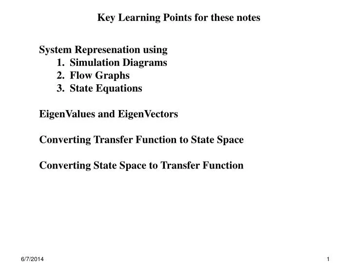
Key Learning Points for these notes. System Represenation using Simulation Diagrams Flow Graphs State Equations EigenValues and EigenVectors Converting Transfer Function to State Space Converting State Space to Transfer Function. 2.7 Simulation Diagrams & Flow Graphs

E N D
Key Learning Points for these notes • System Represenation using • Simulation Diagrams • Flow Graphs • State Equations • EigenValues and EigenVectors • Converting Transfer Function to State Space • Converting State Space to Transfer Function
2.7 Simulation Diagrams & Flow Graphs • Linear Time Invarient System can be represented by • difference equation • transfer function • simulation diagram • flow graphs
i. Shift Register = Delay element ideal delay element shift register ideal delay element E(z) e(k) e(k) z-1E(z) e(k-1) e(k-1) z-1 T transfer function of time delay element = z-1 transform of input: Z[e(k)]=E(z) transform of output: Z[e(k-1)] = z-1E(z) • (1) Simulation Diagram • to obtain Transfer Function (TF) of block diagram use • block diagram reduction • Mason’s Gain Formula basic element of simulation diagrams • continuous systemsintegrator • discrete systems delay element (memory)
input = e(k) ouput = m(k) m(k) = e(k) – e(k-1) - m(k-1) m(k) - e(k) e(k-1) m(k-1) ,…e(2), e(1),e(0) - T=0 T=0 + m(k) ,…m(2),m(1),m(0) e.g.: system represented by difference equation: use ASICs, FPGAs to implement equations with shift registers, adders, summers… • input values: at time t = 0, 2T,4T, … e(kT) = 1 • at time t = 1, 3T,5T, … e(kT) = 0 • outputs: m(k)available at time t=kT (i)initial conditions = 0: set all shift registers to 0 output 0 at k = 0 m(0) = 0 e(0) = 0
Transfer Function:(1+z-1)M(z) = (1-z-1)E(z) - e(k+1) e(k) m(k+1) m(k) ,…e(2), e(1) - e(0) m(0) + m(k+1) ,…m(2),m(1) • (ii) non-zero initial conditions: • replace k with k+1: m(k+1) = e(k+1) – e(k) - m(k) • use shift register for e(k)initialize e(0) • use shift register for m(k) initializem(0) • registers output m(0) and e(0) at k = 0
A B=AG A G B=AG G C=A-B A A 1 C=A-B + - -1 B B • (2) Signal Flow Graph • basic elements are branches &nodes • output signal = branch gain * input signal • signal at a node = sum of all signals from branches coming into node • to obtain TF of signal flow graph use Mason’s Gain Formula
Transfer Function (Mason’s Gain Formula) M1 = - z-1 M2 = 1 L1 = -z-1 = 1 – (L1) = 1 + z-1 1 = 1 2 = 1 M(z) 1 E(z) -z -1 z -1 z-1M(z) 1 -1 T(z) = e.g. m(k) = e(k) – e(k-1) - m(k-1) • Signal Flow GraphBlock Diagram • branch block • node signal • input node input signal • output node output signa
A B C D G3 G1 G2 H1 Massons Gain Formula (review): determine TF from source to sink node • Source Node: (A) signals only flow away from • Sink Node: (D)signals only flow towards • Path: (A, B, C ) sequence of uni-directinal branches • Loop: (B,C, B )closed path • no node is encountered more than one – except return to origin • each branch with and in & out branch • Forward Path:(A, B, C, D ) connects source to sink • Path Gain: (G1,G2,G3) product of transfer functions of all branches in a path • Loop Gain: (G1,H1) product of transfer functions of all branches in the loop • Nontouching Loops: two loops with no nodes in common • Nontouching Loop & Path: loop & path with no nodes in common
T = • 1 - sum(all individual loop gains) • + Σ(product of loop gains of all combinations non-touching loops, 2 at a time) • - Σ (product of loop gains of all combinations non-touching loops, 3 at a time) • + Σ (product of loop gains of all combinations non-touching loops, 4 at a time) … = = T: transfer function Li: loop gain of ith loop Mk: path gain of kth forward path k: value of for part of flow graph not touching kth forward path Determination of TF from Massons Gain Formula
(i) two non-touching loops: • L1 = - G2H1 • L2= - G4H2 • (ii) two forward paths • M1= G1G2G3G4G5 • touches L1& L2 • M2 = G6G5G4 • touches L2 G6 G3 G4 -H1 -H2 • (iii) and i • = 1 – (L1 + L2 ) + (L1L2 ) • i=of flow graph without Mi(and any nodes) • 1=1 • 2= 1-L1 T = G6 G1 G2 G3 G4 G3 G2 G1 G5 -H1 -H2 R(s) C(s) -H1 -H2 e.g. TF from Signal Flow Graph
m(k) + an-1m(k-1)+…+ a0m(k-n) = bn e(k) + bn-1e(k-1)+…+ b0 e(k-n) (2.41) e(k) e(k-1) e(k-2) e(k-3) e(k-n) T T T m(k) T M(z) + an-1 z-1 M(z)+…+a0 z -n M(z) = bn E(z) +…+b0 z-nE(z) bn bn-1 bn-2 b0 (1 + an-1 z-1 +…+a0 z -n )M(z) = (bn + bn-1 z-1+…+b0 z-n )E(z) (2.42) + + + + + + m(k) m(k-1) m(k-n) T T (2.43) - - - an-1 an-2 a0 General nth order diffence equation Non-minimal representation: minimal representaion has ndelay elements
Example of minimal simulation diagram • determining the transfer function • m(k) = y(k) – y(k-1) M(z) = (1-z-1)Y(z) • y(k) = e(k)-y(k-1) E(z) = (1+z-1)Y(z) + - y(k-1) e(k) y(k) T + - m(k) • Masons Gain Formula • M1 = - z-1, M2 = 1 • L1 = -z-1 • = 1 + z-1 • 1 = 1 • 2 = 1 1 z-1Y(z) Y(z) E(z) M(z) z-1 -1 1 1 -H1 T =
transfer function u(k) E(z) x(k) G(z) M(z) y(k) state variables x1(k) x2(k) xn(k) ith external input, ui(k) input space =u(k) hth system output, yh(k) output space = y(k) State Variable Method jth internal state variable,xj(k) state space = x(k) state vector u1(k) u2(k) ur(k) y1(k) y2(k) yp(k) 2.8 State Variables system representation • for any inputu(k) represents minimal information needed to determine • future statesx(k+1) • system outputsy(k)
(1) non-linear, time varying system (k implies kT) system description at t = k+1 x(k+1) = f [x(k),u(k)] (2.45) system response at t = k y(k) = g [x(k),u(k)] (2.46) (2) linear, time varying system system description at t = k+1 x(k+1) = A(k)x(k) + B(k)u(k) (2.47) system response at t = k y(k) = C(k)x(k) + D(k)u(k) (2.48) (3) linear, time invarient system system description at t = k+1 x(k+1) = A x(k) + B u(k) (2.49) system response at t = k y(k) = C x(k) + D u(k) (2.50)
e.g. y(k+2) = u(k) + 1.7y(k+1) – 0.72y(k) x1(k) = y(k) x2(k) = y(k+1) = x1(k+1) x1(k+1) = x2(k) x2(k+1) = u(k) + 1.7x2(k) – 0.72x1(k)
G(z) = (2.51) for input u(k) and output y(k) = G(z) = (2.52) Y(z) = (bn-1z n-1 + bn-2 z n-2+…+ b0 z ) E(z) (2.53) U(z) = (zn + an-1 z n-1 +…+ a1z + a0)E(z) (2.54) Dervation of state-space equations from TF - Control Canonical Form (i) start with transfer function G(z)
(iii) Define State Variables • x1(k) = e(k) • x2(k) = x1(k+1) = e(k+1) • x3(k) = x2(k+1) = x1(k+2) = e(k+2) • x4(k) = x3(k+1) = x2(k+2) = x1(k+3) = e(k+3) • … • xn(k) = xn-1(k+1) = e(k+n-1) (2.55) • (ii) From Real Translation property • E(z) e(k) • zE(z) e(k+1) • zn E(z) e(k+n) …
(iv) obtain state equations for Control Canonical Form • x1(k+1) = x2(k) • x2(k+1) = x3(k) • … • xn(k+1) = -a0 x1(k)- a1 x2(k)- a2 x3(k) - …- an-1 xn(k) + u(k) • from (2-55) xn(k+1) = e(k+n) from (2-54) u(k) = e(k+n) + an-1e(k+n-1) +…+ a1 e(k+1) + a0e(k) e(k+n) = u(k) - an-1e(k+n-1) -…- a1 e(k+1) - a0e(k) xn(k+1) = u(k) - an-1xn(k) -…- a1 x2(k) - a0x1(k)
(2.59) x(k+1) = Ax(k) + Bu(k) y(k) = Cx(k) (2.60) State Space Equation • eqn (2.51) = transfer function representation • eqn (2-59) & (2-60) = state equations
Multiply 2.51 by z-n TF of delay ofnT seconds isz-n = G(z) = (2.61) Y(z) = (bn-1z -1 + bn-2 z -2+…+ b0 z-n ) E(z) (2.62) U(z) = (1 + an-1 z -1 +…+ a1zn-1 + a0 z-n)E(z) (2.63) E(z) = U(z) - (an-1 z -1 +…+ a1zn-1 + a0 z-n)E(z) (2.64) Derive signal flow graph for control canonical form use dummy variable, E(z)
Y(z) bn-1 bn-2 b1 b0 U(z)1 E(z) z-1E(z) z-2E(z) z-nE(z) z-1 z-1 z-1 -an-1 -an-2 -a1 -a0 Y(z)= bn-1z -1 E(z) + bn-2 z -2 E(z)+…+ b0 z -n E(z) (2-62’) E(z) = U(z) - an-1 z -1 E(z)+…+ a1z 1-n E(z) + a0 z –n E(z)(2-64’)
y(k) + bn-1 bn-2 b1 b0 u(k) e(k) e(k-1) e(k-2) e (k-n+1) e(k-n) + T T T T xn(k) xn-1(k) x1(k) x2(k) -an-1 -an-2 -a1 -a0 derive simulation diagram for control canonical form from signal flow
u(k) b0 b1 bn-2 bn-1 + + - + + - + - + + - y(k) T T T T a0 a1 an-2 an-1 (v) observer canonical form
U(z) b0 b1 b2 bn-1 Yz) E(z) z-1 z-1 z-1 -an-1 -a2 -a1 -a0 signal flow graph forobserver canonical form from
u(k) b0 b1 bn-2 bn-1 + + - xn(k) xn-1(k) + + - + - + + - x2(k) y(k) T T T T x1(k) a0 a1 an-2 an-1 • derive State Space for observer canonical form x1(k+1) = x2(k) - an-1x1(k) + bn-1u(k) x2(k+1) = x3(k) - an-2x1(k) + bn-2u(k) … xn-1(k+1)= xn(k) - a1x1(k) + b1u(k) xn(k+1) = - a0x1(k) + b0u(k) and y(k) = x1(k)
thus State Space Represenation for observer canonical form x(k) + u(k) x(k+1) = y(k)= [1 0 0 … 0 ] x(k)
G(z) = x(k+1) = y(k)= 1 z-1 Yz) z-1 1 z-1 1 2 U(z) X3 X2 X1 -2 -1 -0.5 y(k) u(k) T T T x3(k) x2(k) x1(k) -2 -1 -0.5 + 2 1 1 + e.g. 2.17 state = output of delay
Y(z) b2 b1 b0 X2 X1 U(z) 1 z-1 z-1 -a1 -a0 x(k+1) = x(k) + u(k) wrong! – only 2 state variables y(k) = [b0 b1 b2 ]x(k) G(z) = e.g. numerator & denominator with same order Direct path from Y(z) to E(z) x1(k) = e(k-2) x2(k) = x1(k+1) = e(k-1) x2(k+1) = u(k) – a1 x2(k) –a0 x1(k) from signal flow graph: Y(z) = b2E(z) + b1X2(z) + b0X1(z) E(z) = U(z) - a1X2(z) – a0X1(z) thus Y(z) = b2U(z)+ (b1-b2a1)X2(z) + (b0– b2a0)X1(z) and y(k) = [(b0–b2a0) (b1- b2a1)] x(k) + b2u(k)
x1(k) = e(k-n) x2(k) = x1(k+1) = e(k-n+1) x3(k) = … G(z) = y(k) + b1 b0 e(k) u(k) x2(k) x1(k) T T + a1 a0 Deriving State Models: (1) from transfer function: • (2) from Simulation Diagram • assign a state variable to each delay output • derive delay input & system output in terms of delay output& system input
Deriving State Models (continued) • (3) Decompose High Order TF, G(z) into product of simpler TFs • G(z)= G1c(z)G2c(z)…Gnc(z) • realize Gic(z) by either technique (1) or (2) • connect Gic(z)’s by cascading them • use 2nd orderGic(z)’s to avoid complex poles • (4) Decompose High Order TF, G(z) into sum of Simpler TFs • G(z) = G1p(z) + G2p(z) +…+ Gnp(z) • realize Gip(z) by either technique (1) or (2) • connect Gic(z)’s in parallel
2.9 Other State-Variable Formulations • Transfer Function: • gives system input/output relationship • unique for a given system • State Model: • gives internal system description (not unique) • gives input/output relationship • derived from transfer function, difference equation, simulation diagram
x(k) + u(k) x(k+1) = • (1) State Space from TF • y(k+2) = u(k) + 1.7y(k+1) - 0.72y(k) (derived earlier) y(k) = [1 0] x(k)
y1(k) = x1(k) x1(k+1) = u(k)+0.9x1(k) y(k) u(k) + + T T x2(k) x1(k) y2(k) = x2(k) x2(k+1) = u’(k)+0.8x2(k) u’(k) = x1(k) 0.9 0.8 overall state model: x(k+1) = x(k) + u(k) y(k) = [0 1]x(k) (2) Decompose G(z) into product of simpler TFs
u(k) x1(k) + T 10 y(k) 0.9 + x2(k) T -10 + 0.8 overall state model: x(k+1) = x(k) + u(k) y(k) = [10 -10]x(k) (3) Decompose G(z) into sum of simpler TFs (partial fraction expansion) y(k) = 10x1(k) x1(k+1) = u(k) + 0.9x1(k) y'(k) = -10x2(k) x2(k+1) = u(k) + 0.8x2(k)
a11 a12 a13 a11 a12 a21 a22 a23 a21 a22 a31 a32 a33 a31 a32 Review of Matrices (1) trace tr(A) = sum of elements on diagonal (a11 + a22 +…+ ann) • (2) determinant|A| = () a1j1, a1j 2, …, a1jn • summation over all permutations j1, j2, j3, …jn of set S={1...n} • ‘+’ for even permutation, • ‘-‘ for odd permutation |A| = a11a22a33 + a12a23a31 + a13a21a32 - a11a23a32 - a12a21a33 - a13a22a31 • determinant of 22 square matric A, |A| = a11a22 – a12 a21 • (3) eigenvalues |zI - A| = 0 • determinant of 2nd order system: (z-a11)(z-a22) – a12 a21 = 0 • eigenvaues are roots of z2 – (a11 + a22)z + (a11 a22 – a12 a21) (4) eigenvectors if zi is an eigen value of A an eigenvector xi satisfies zixi = Axi
for 22 square matrice A Adj A = inv(A) =
Similarity Transformation of State Model • x(k+1) = Ax(k) + Bu(k) (2-67) • y(k) = Cx(k) + Du(k) • asume x and w are1 n state vectors • let Pbe an n n non-singular matrice • apply linear transformation to x(k) • x(k) = Pw(k) (2-68) x1(k) = p11w1(k) + p12w2(k) + …p1nwn(k) x2(k) = p21w2(k) + p22w2(k) + …p2nwn(k) … xn(k) = pn1w1(k) + pn2w2(k) + …pnnwn(k) • each unique, non-singularPyields a different state model
Similarity Transformation of State Model (continued) substitution of (2-68) into (2-67) yields: w(k+1) = P-1APw(k) + P-1Bu(k) y(k) = CPw(k) + Du(k) let Aw= P-1AP Bw = P-1B Cw = CP Dw= D then w(k+1) = Aw w(k) + Bw u(k) y(k)= Cw w(k) + Dw u(k)
|zI-A|= • = (z-a11)(z-a22) - (a12a21) • = (z -z1)(z-z2) • Characteristic Equationof A determinant: |zI-A|=0 Eigenvalues:roots of characteristic equation • aka characterisitc values if zi are eigenvalues of A |zI-A| = (z-z1) (z-z2)…(z-zn)=0 • |zI-A| determines stability for system • not unchanged by lineat transformation: |zI-A| = |zI-Aw|
Givren Similartiy Transform: Aw= P-1AP (i) eigen values, ziare unchanged (ii) |Aw| = | P-1AP| = | P-1||A| |P| = | P-1||P| |A| =|A| (iii) trace: tr Aw =tr A = z1 + z2 +…+ zn (iv)C[zI-A]-1 B + D = Cw [zI-Aw] -1 Bw + Dw
If a system has distinct eigenvalues it is possible to derive a state variable model with diagonal system matrix • assume a vector mi and a scaler zi given as • mi= [m1i, m2i, …, mni]T • Ami = zimi Eigenvalues and Eigenvectors
Eigenvalues and Eigenvectors (continued) • if (ziI – A)mi= 0 has a nontrivial solution then |ziI – A| = 0 and • ziis eigenvalue of A • miis called an eigenvectorof A • with n eigenvectors we have the modal matrix, M = [m1 m2 …mn ] A[m1 m2 …mn ] =AM = [m1 m2 …mn ]zI the diaganol matrix, is given as = M-1AM
x(k) + x(k+1) = u(k) y(k)= x(k) • setting Ami = zimifor z1 = 0.8, z2 = 0.9yields 0.8m11 + m21 = 0.8m11 0.9m21 = 0.8m21 thus m11 = arbitrary and m21= 0 0.8m12 + m22 = 0.9m12 0.9m22 = 0.9m22 thus m22 arbitrary and m12 = 10m22 • eigenvectors of A are given as: = m2= m1= e.g. characteristic eqn: |zI-A| = 0 (z-0.8)(z-0.9) = 0 eigenvaluesgiven asz1 = 0.8, z2 = 0.9
M = and diagonal system matrix is given as M-1 = inv(M) = = = = M-1 A M = = = Bw= M-1B = Cw= CM = [1 0] = [1 10] w(k+1)= w(k) + u(k) y(k) =[1 10]w(k) e.g. letting p = q =1 we have the modal matrix is given as: by similarity transform we have
2.10 Obtain Transfer Function from State Model • (1) Given state space equations construct simulation diagramor signal flow graph • obtain difference equation relationship take z-transform • obtain transfer function from reductionor Mason’s gain formula (2) take z-transform of state equations & eliminate state varible, x x(k+1) = Ax(k) + Bu(k) zX(z) – zx(0) = AX(z) + BU(z) y(k) = Cx(k) + Du(k) Y(z) = CX(z) + DU(z) • assume initial condition = 0 • [zI –A]X(z) = BU(z) • X(z) = [zI –A]-1BU(z) thenY(z) = [C [zI –A]-1B + D] U(z) and transfer function:G(z) = C [zI –A]-1B + D
2.11 Solutions of State Equations state equations given as: x(k+1) = Ax(k) + Bu(k) y(k) = Cx(k) + Du(k) x(1) = Ax(0) + Bu(0) and we have • x(2) = Ax(1) + Bu(1) • = A(Ax(0) + Bu(0)) + Bu(1) • = A2x(0) + ABu(0) + Bu(1) x(3) = Ax(2) + Bu(2) = A(A2x(0) + ABu(0)) + Bu(1)) + Bu(2) = A3x(0) + A2Bu(0) + ABu(1) + Bu(2) • (1) Recursive Solution - assume time invarient system with: • x(0) • and u(j) j=1,2,3…known x(k) = Akx(0) + Ak-1-iBu(i) (2.88) thus Ak-1-iBu(i) + Du(k) y(k) = CAkx(0) +C
Recursive Solution (continued) definestate transition matrixor fundamental matrix as: (k) = Ak x(k) = (k) x(0) + (k-1-i)Bu(i) (2.89) y(k) = C(k)x(0) + C(k-1-i) Bu(i) • Properties of (k) • x(k) = (k) x(0) (0) = I • (k1 + k2) = Ak1+k2 = Ak1 Ak2 = (k1)(k2) • (-k) = A-k = [Ak]-1 = -1(k) • (k) = -1(-k)
2. z-transform method x(k+1) = Ax(k) + Bu(k) y(k) = Cx(k) + Du(k) • if we assumeu(k)= 0 then zX(z) - zx(0)= AX(z) • (zI-A)X(z) - zx(0) = 0 • X(z) = z[zI-A]-1x(0) • then x(k) = Z-1{X(z)} • = Z-1{z[zI-A]-1x(0)} • if u(k) = 0 x(k) = (k) x(0) from (2.89) then (k) x(0) = Z-1{z[zI-A]-1x(0)} thus substitute (k) = Z-1{z| zI-A|-1 }
G(z) = x(k+1)= x(k) + u(k) e.g. derive State Equations: u(k)= e(k+2)+3e(k+1)+ 2e(k) y(k) = e(k+1) + 3e(k) x1(k) = e(k) x2(k) = e(k+1) x2(k+1) = u(k) - 3x2(k) - 2x1(k) y(k) = [3 1]x(k)
x(0) + u(0) = x(1) = y(1) = y(2) = y(3) = [3 1]x(1) = 1 [3 1]x(2) = 1 [3 1]x(2) = -1 x(1) + u(1) = x(2) = x(2) + u(1) = x(3) = asssume system is initially at rest (x(0) = 0 ) & input is unit step: u(k)= 1