Download
1 / 12
130 likes | 201 Views
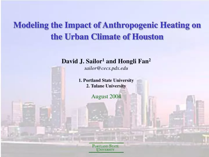
Modeling the Impact of Anthropogenic Heating on the Urban Climate of Houston. David J. Sailor 1 and Hongli Fan 2 sailor@cecs.pdx.edu 1. Portland State University 2. Tulane University August 2004. Q sw. Q. Q f. time. Motivation. On average anthropogenic heating (Q f ) is small

E N D
Modeling the Impact of Anthropogenic Heating on the Urban Climate of Houston David J. Sailor1 and Hongli Fan2 sailor@cecs.pdx.edu 1. Portland State University 2. Tulane University August 2004
Qsw Q Qf time Motivation • On average anthropogenic heating (Qf) is small • peak solar flux is ~1000 W m-2 in summer • city-scale, daily average Qf is ~ 30 to 50 Wm-2 • Local peaks in anthropogenic heating can be a factor of 10-20 higher than the city-scale average value*. • In morning/evening Qf may affect boundary-layer transitions and mixing processes with important AQ implications * Sailor, D.J., and L. Lu, (2004) “A Top-Down Methodology for Developing Diurnal and Seasonal Anthropogenic Heating Profiles for Urban Areas,” Atmospheric Environment, 38 (17), 2737-2748.
(vehicles) (building sector) (metabolism) population density [person/km2] non-dimensional traffic profile [-] vehicle energy used per unit distance [W km-1] distance traveled per person [km] metabolic heat per person [W] electricity profile [-] electricity consumption [W] heating fuel profile [-] heating fuel consumption [W] A top-down methodology for Qf Determine consumption rates separately for residential, commercial, and industrial sectors. For further details see poster P3.6
Estimating population density • Census Transportation Planning Package (CTPP*) • Need: population data from the basic census database underestimate daytime populations by ~ a factor of 2 at the city scale… • CTPP data available at range of scales (city, census tract, TAZ) • Residents, non-working residents, workers, time-of-arrival data… • Estimate nighttime and daytime (workday) populations • Neglect other visitors to city (hotel/conference/shoppers/etc) * www.bts.dot.gov
Anthropogenic Heating in Houston at Various Scales • Workday population density (centered on CBD) • 1,538 persons/km2 at city scale • 20,844 persons/km2 at census tract scale • up to 184,500 persons/km2 at TAZ scale • Since Qf scales with population density it can vary dramatically depending upon the scale of analysis
Day (summer) Night (summer) Anthropogenic Heating in Houston at TAZ Scales
In this study… we define 3 categories of urban land use and implement one distinct Qf profile for each category. High spatial resolution case: Q1 Houston Summer City-average (low spatial resolution case: Q2)
Simulation Overview • MM5 implementation: • Modified USGS land use with 3 new urban subcategories • No urban canopy parameterization • Diurnal land-use-dependent profile for Qf • Qfinput into near-surface air layer as DT • Modified Blackadar PBL scheme • 4 two-way nests, 1km grid cells in inner domain • Simulation Episodes: • Aug. 30, 2000 • Sept. 27, 2002 • Q0 – No anthropogenic heating • Q1 – Land-use specific profiles • Q2 – Single city-scale avg. profile.
Temperature Perturbation (avg. over city) Morning (6am) Day (noon) Night (8pm) 092702 083000 Q1 – Q0: Near-surface air temperature difference between base case (no Qf) and spatially-detailed Qf case (~ 2-2.5 0C during night/morning, ~ 0.25-0.5 0C during day)
Q1 – Q0: Near-surface air temperature difference between base case (no Qf) and spatially-detailed Qf case (~ 2-2.5 0C during night/morning, ~ 0.25-0.5 0C during day) 092702 45 10 10 45
9am 5pm 11am 7pm Sept. 27, 2002 simulation Q1 – Q 2: Temp. difference between spatially-detailed Qf case and city-average Qf case: (DT ~ 0.5-2.0 oC during transitions; 0.2-0.4 oC during day ) Vertical cross section (0-2.5km)
Conclusions and Future Work • Qf in Houston is 30-50 W/m2 at the city scale, but may be a factor of 10 to 20 larger in isolated regions within the core of the city. • CTPP data are useful for population-based analyses of anthropogenic heating (and moisture), but refinements & extensions are possible. • Addition of Qf in MM5 creates a summer heat island signature in morning and night (~ 2.0 oC ) , with less impact during day ( ~ 0.25-0.5 oC ). • Including Qf at high spatial resolution can generate local temperature perturbations of up to several degrees C compared with use of city-average profiles. Effect is largely limited to morning/evening transition hours. • Next steps include: • use improved landuse database and refined surface characteristic definitions • better vertical representation of Qf in MM5 • workday vs. non-workday profiles • integration with an urban canopy parameterization • investigate winter episodes sailor@cecs.pdx.edu www.cecs.pdx.edu/~sailor