Download
1 / 53
580 likes | 922 Views
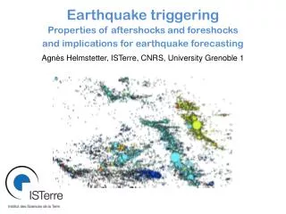
Earthquake triggering Properties of aftershocks and foreshocks and implications for earthquake forecasting Agnès Helmstetter , ISTerre , CNRS, University Grenoble 1. Earthquake triggering. When? Where? What size? Scaling with mainshock size? How ?…. Outline Aftershocks

E N D
Earthquake triggering Properties of aftershocks and foreshocks and implications for earthquake forecasting AgnèsHelmstetter, ISTerre, CNRS, University Grenoble 1
Earthquake triggering When? Where? What size? Scaling with mainshock size? How?…
Outline Aftershocks when? where? scaling with mainshock size? why? : static, dynamic, or postseismic stress change? model? : ETAS or rate & state Foreshocks Earthquakes that trigger by chance a larger event … or part of the nucleation process? Distribution in time, space and magnitude and comparison with ETAS
1yr 1 day Foreshocks and aftershocks of Landers, California M=7.3 M=6.5 1992/4/23 Joshua-Tree m6.1 Foreshocks a few hrs before Landersm≤3.6 1992/6/28 Landers m7.3
Japan M=9.1 Sumatra M=9.0 m=7 California Temporal decay of aftershocks m=2 Omori p=0.9 • stacks for California and rate following the Sumatra and Tohoku M=9 EQs • aftershock rate ~1/tp with p≈0.9 (Omori’s law) • duration ≈ yrs indep of M
Japan M=9.1 Sumatra M=9.0 Scaling with mainshock magnitude N(M)~10M California 2<M<7.5 • Aftershock rate N(M)~10M ~ rupture area • Magnitude distribution P(M)~10-M (GR law) • Small and large EQs have the same influence on EQ triggering !
7<m<7.5 - aftershocks 1 day after -- background 1 day before number of aftershocks 2<m<2.5 distance from mainshock hypocenter (km) • relocated catalog for Southern California • [Shearer et al., 2004] • average distance • ≈ rupture length L • <d> ≈ 0.01x10m/2 km • max distance ‘+’ dmax ≈ 7 L ≈ 0.07x10m/2 km Aftershocks : Where?
mainshocks 7<m<7.5 b=1 mainshock 2<m<2.5 Aftershocks : What size? • aftershocks magnitude distribution = GR law • aftershock size does not depend on the mainshock magnitude !
Seismicity remotely triggered by M7.3 Landers EQ [Hill et al 1993] Long Valley Geysers Parkfield Dynamic triggering unfiltered filtered 5-30 Hz • Mostly in geothermal or volcanic areas • Dynamic stress change ≈ 1 bar >> static • During seismic wave propagation • but also in the following days • Transient deformation at Long-Valley : • change in fluid pressure ?
Summary of observations about aftershocks • aftershock rate decays as N~1/t, for t between a few sec and several yrs, independently of M • + short-term remote dynamic triggering by seismic waves • number of aftershocks increases as N ~10M~ L2, for 0<M<9. • small EQs collectively as important as larger ones for triggering • the size of a triggered EQ is not constrained by M • typical triggering distance ≈ L ≈ 0.01x10m/2 km, • max distance for t<1day ≈ 7L
Triggered seismicity : not only aftershocks! • Other evidences of triggered seismicity, natural and human-induced • rainfall (pore pressure changes due to diffusing rain water) [Hainzl et al 2006] • CO2 degassing [Chiodini et al 2004; Cappa et al 2009] • slow slip events [Segall et al 2006; Lohman & McGuire 2007, Ozawa et al 2007] • tides (hydrothermal, volcanic areas or shallow thrust EQs, ∆≈10 kPa, ∆R=10%)[Tolstoy et al 2002 ; Cochran et al 2004] • migration of underground water or magma [Hainzl & Fisher 2002] • nuclear explosions [Parsons & Velasco 2009] • mining (stress concentrations due to the excavation)[McGarr et al., 1975] • dams (filling of water reservoirs)[Simpson et al 1988, Gupta 2002] • fluid injections or extraction (geothermal power plants, hydraulic fracturing, for oil and gas production, injection of wastewater, extraction of groundwater) [McGarr et al., 2002; Gonzales et al 2012; Ellsworth 2013] • … any process that modifies the stress or the pore pressure
≈yrs time time time seismicity rate after a mainshock R What triggers aftershocks? Aftershocks triggered by Static stress changes? postseismic? dynamic? Coseismic, permanent afterslip, fluids seismic waves σ σ σ ≈yrs time ≈sec
Static stress change permanent change⇒easy to explain long-time triggering fast decay with distance ~ 1/r3⇒how to explain distant aftershocks? Dynamic stress change short duration⇒how to explain long time triggering? slower decay with distance ~ 1/r⇒better explains distant aftershocks Postseismic relaxation afterslip, fluid flow, viscoelastic relaxation slow decay with time, ~ seismicity rate ⇒ easy to explain Omori law but smaller amplitude than coseismic stress change Mechanisms of aftershocktriggering
Statistical model : ETAS seismicity rate = background+ triggered seismicity[Kagan, 1981, Ogata 1988…] R(t,r) = µ(r) + ∑ti<tϕ(t-ti, |r-ri|, mi) Physical model : coulomb stress change calculations + rate & state model A ≈ 0.01 parameter of R&S friction law, increase of friction with V σ: normal stress ; τ: coulomb stress change ;τr’tectonic stressing rate r : background seismicity rate for τ’=τr’ ; N : cumulated number∫R(t)dt [Dieterich 1994] Modellingtriggeredseismicity
space time space time ETAS model Input : proba that an EQ (t,r,m) triggers another EQ(t’,r’,m’) Results : multiple interaction between EQs
R(t) Aftershocks « direct » Omorilaw Rd(t) ~1/tp t mainshock <R(t)> t mainshock ETAS : aftershocks and foreshocks (t) • Assumptions: • Results Aftershocks +aft. of aft. + … « global » Omorilaw Rg(t) » Rd(t) Rg(t) ≈ 1/tpgwthpg<p Foreshocks Inverse Omori law R(t) ~1/tpf pf<p
Foreshocks inverse Omori law N(t)~1/(t+c)pfwith pf≤ p Aftershocks, Omori law N(t)~1/(t+c)p seismicity rate background rate time mainshock “Foreshocks”, “mainshocks”, “aftershocks” average over many sequences ---- a typical sequence
ETAS model : main results • Aftershocks • “Global” Omori law with a pglobal≤ pdirect • Bath’s law : largest aftershock average magnitude = M-1.2 • Diffusion of aftershocks • Foreshocks • Inverse Omori law with pforeshocks≤pdirect • Rate of foreshocks independent of mainshock magnitude (if any EQ is a mainshock) • Deviation from GR law bforeshocks≤b • Migration toward mainshock
τ(t) R(t) T» ta R(t) T«ta Rate-and-state : periodic stress changes • stress : τ(t) = cos(2πt/T) + τ’r t • T« ta or T»ta • ta : nucleation time ≈ yrs slow short-times regime for T«ta R~R0exp(τ/Aσ) tides, seismic waves long-times regime for T»ta R~dτ/dt tectonic loading fast
Rate-and-state : triggering by a stress step • Reproduces Omori law withp=1for a positive stress change • Requires a very large ∆ : c=10-4 ta=100 days Aσ=1 MPa⇒∆=15 MPa ! triggering quiescence
Heterogeneity of EQ source and aftershocks • Planar fault with uniform stress drop slip∆ EQ rate • Real faults : heterogeneous slip and rough faults • >hetergoneousstress change in the rupture zone • > most aftershocks on or very close to the rupture zone slip ∆ EQ rate [Marsan, 2006; Helmstetter & Shaw, 2006]
mean stress τ0 Slip and shear stress heterogeneity, aftershocks Modified « k2 » slip model: U(k) ~ 1/(k+1/L)2.3 [Herrero & Bernard, 1994] aftershock map synthetic catalog R&S model shear stress stress drop τ0 =3 MPa slip
∆(MPa) x(km) R&S model, stress heterogeneity, and aftershock decay with time Aftershock rate heterogeneous ∆ ∆/As=10 ∆/As=-10 Heterogeneous • triggering at short-timet«ta : Omori law with p<1 • quiescence at long time (t≈ta≈yrs) • [Marsan, 2006; Helmstetter and Shaw, 2006]
Modified k2 slip model, off-fault stress change • fast attenuation of high frequency τ perturbations with distance d L coseismic shear stress change (MPa)
Modified k2 slip model, off-fault aftershocks • seismicity rate and stress change as a function of d/L • quiescence for d >0.1L d L standard deviation average stress change
R&S and aftershock time decay • stacked A.S. for 82 M.S. with 3<M<5 z<50 km in Japan • triggering following Omori law decay for 10 s <t<1 yr with pincreasing slightly with time [Peng et al 2007] Data Fit by rate-state model with a Gaussian stress pdf <∆τ> =0 std(∆τ)/An = 11 ta= 0.9 yrs p=1 ta
Modeling aftershock rate with R&S model and heterogeneous static stress change Sequence pτ* (MPa)ta (yrs) Morgan Hill M=6.2, 1984 0.68 6.2 78. Parkfield M=6.0, 2004 0.88 11. 10. Stack, 3<M<5, Japan* 0.89 12. 1.1 San Simeon M=6.5 2003 0.93 18. 348. Landers M=7.3, 1992 1.08** 52. Northridge M=6.7, 1994 1.09** 94. Hector Mine M=7.1, 1999 1.16** 80. Superstition-Hills, M=6.6,1987 1.30 ** ** *[Peng et al., 2007] **we can’t estimate τ* becausep>1
R(t) τ(t) time time R&S : triggering by afterslip Mainshock ⇒ coseismic stress change ⇒ afterslip ⇒ postseismicreloading ⇒ aftershocks? AfterslipPostseismic Aftershock rate stress change V(t) time
R&S : triggering by afterslip We assume stressing rate due to afterslipdτ/dt~ τ’0/(1+t/t*)qwithq=1.3 seismicity rate stressing rate • Apparent Omoriexponent p(t) decreasesfrom 1.3 to 1
R&S model and Omori’s law Deviations from Omori law with p=1 can be explained by : Coseismictriggering with heterogeneous stress step • short-time triggering p≤1, p↘ with t and with stress heterogeneity • long-time quiescence Postseismic triggering by afterslip • Omori law decay with p< or >1 τ(x,y) τ(t) τ(t) p=1 log R log R r r p=1 log t log t
EQ triggering and EQ forecasting • seismicity rate increases a lot (≈104) after a large EQ • … but the proba of another large EQ is still very low ! • limited use for EQ forecasting ? • Methods : statistical (ETAS, STEP, kernel smoothing …) or physical models (R&S + Coulomb stress change) • ETAS generally provides the best forecasts [Woessner et al 2011; Segou et al 2013] • Very simple to use (requires only t,x,y,z,m) • Bad modeling of early A.S. spatial distribution • … but can be corrected (kernel smoothing of early A.S.) [Helmstetter et al 2006] • Coulomb-stress change with R&S • Good fit in the far-field, but bad near the rupture (∆ is not accurate) • … but can be corrected by assuming a pdf of ∆[Hainzl et al 2009] • Usually include only M>6 M.S. (with known slip)
Increase of seismic activity before mainshock • … on average • Part of the nucleation process ? • Or cascading triggering process ? And before the mainshock?
Example : seismicity rate before each M>7 mainshock in California and stack for all M>5 (for R<20 km) Seismicity rate before mainshock
Stacks for California and ETAS for mainshock with 2<M<7.5 • Mainshock : any EQ not preceded by a larger EQ for T=100 days and r<10 km • Foreshocks : EQs within 100 days before and 10 km • Power-law ↗ of seismicity : inverse Omori law • Number of foreshocks ↗ with M because of mainshock selection rules • California ETAS Seismicity rate before a mainshock p=0.8 p=0.8
Stacks for California and ETAS for mainshock with 2<M<7.5 • For small mainshocks : roll-off Mforeshock<Mmainshock • For large mainshocks : increase in the rate of large EQs • ETAS theory : P(m)= GR(m,b) + GR(m,b-α) [Helmstetter et al 2003] • California ETAS Magnitude pdf of foreshocks
Stacks for California and ETAS for mainshocks with 2<M<7.5 (SHLK catalog) • California ETAS Spatial distribution of foreshocks (M) • small d : similar pdf(d) for all M, but ! location error ↗ with M • large d : increase in pdf(d) for all M due to selection rule MF.S. < MM.S.
Stacks for California and ETAS for mainshocks with M>4 • California ETAS timebefore M.S. (day). Spatial distribution of foreshocks (time) • apparent migration towardmainshock.
Swarms sometimes detected before mainshocks (not explained by ETAS) ex : M=9 Tohoku [Marsan et al, 2013] • «Repeating» EQs (triggered by aseimic slip?) and low-frequency noise • ex : m=7.6 Izmit[Bouchon et al 2011] or M=9 Tohoku [Kato et al 2012] • Slow slip event • Ex : M=8.1 Iquique [Ruiz et al, 2014] • Accelerating foreshock sequences followed by enhanced aftershock rate • Stack of M>6.5 mainshocks worldwide [Marsan et al 2014] • Foreshock / aftershock ratio istoo large • Stack for 2.5<M<5.5 mainshocks in California [Shearer 2012] • Foreshocks do not promote the mainshock (∆<0) • Landers M=7.3 and other EQs in California M4.7-6.4 [Dodge et al 1995,1996] • Accelerating slip predicted by R&S friction law and lab friction experiments … but very small slip (≈ Dc) and difficult to detect [Dieterich 1992] Foreshocks = asesimic loading ?
but in most cases nothing special occurs before mainshocks • and most slow EQs, repeating EQs or swarms are not followed by mainshocks ! • need to consider whole seismicity (not only before mainshocks) to check that these patterns are really unusual ! Asesimic loading before mainshocks?
fitting seismicity with ETAS with variable background µ(t,r) to detect deviations = transient [Marsan et al, 2013] • Transient before • Tohoku, Jan-Feb/2011 • ≈30 days, 40 km • ●all EQs • ●transient • but several other swarms detected not related to large EQs … Swarms before mainshocks
accelerating repeating EQs with very similar waveforms during the last 44 mn before M=7.6 1999 Izmit EQ [Bouchon et al 2011] • 18 events with 0.3<M<2.7, distant by <20 m Repeating EQs before mainshocks Normalized waveforms, chronological order Waveforms of the 1st and 2nd ev. Top : filter <3 Hz
migrating foreshocks and repeating EQs before M9.0 Tohoku [Kato et al 2012] Repeating EQs before mainshocks • repeating EQs : large correlation -> same exact location?
Intense foreshock activity and a SSE before M=8.1 Iquique [Ruiz et al 2014] Slow slip events before mainshocks M8.1 M6.7 SSE with slip≈1m following the largest M6.7 foreshock 15 days before mainshock (or unusually large afterslip?)
Stacked seismicity rate with M>4 before and after M>6.5 mainshocks in the worldwide ANSS catalog [Marsan et al 2014] • Population A : • Significant precursory • acceleration • Population B : • No significant precursory • acceleration • This pattern cannot be explained by ETAS, incompleteness, or # in M.S. M • episodic creep that preceded the M.S. and lasted during the A.S. sequence? Foreshock activity related to enhanced aftershocks
M7.3 mainshock Stress change due to the Landers foreshocks did not trigger the mainshock (∆<0)… but results depend on relocation method M7.3 mainshock Foreshocks did not trigger each other and did not trigger the mainshock? M3.6 foreshock M3.6 foreshock [Marsan 2014] SHLK catalog M3.6 foreshock In SHLK catalog [Dodge et al 1995]
Conclusion • earthquake triggering explains most properties of EQ catalogs • triggering mechanism : static? dynamic? postseismic? • but some discrepancies : swarms, heterogeneity, excess of foreshocks … • need to model accurately «normal» seismicity to detect deviations • deviations from normal seismicity ⇒ aseismic loading? • detection of “aseismic loading” : from EQ catalogs? Geodesy? • aseismic loading = precursor (part of nucleation)? • or aseismic loading = potential triggering factor (like foreshocks)? • implication for EQ forecasting : • ↗ in seismicity rate ⇒ ↗ in the proba of a future large event? • Or can we do better?
Tutorial : statistical analyses of EQ catalogs to reveal nucleation and triggering patterns • distribution of aftershocks and foreshocks in time, space and magnitude • transient increase in catalog incompleteness after a large EQ, implication for the temporal decay of aftershocks • how to identify foreshocks, mainshock and aftershocks? • comparison of foreshocks and aftershocks properties in ETAS model or in the R&S model • can we estimate ETAS model parameters (p, c, α, µ, b …) from stacked aftershock sequences? • how dependent are the results on : parameter choices (windows in time, space, magnitude …), location errors, catalog incompleteness …?
Tutorial • download and unzip • ftp://ist-ftp.ujf-grenoble.fr/users/helmstea/CARGESE.zip • Archive with EQ catalogs, matlab codes, ETAS program • You alsoneedmatlab and a fortran compiler to use the ETAS simulator
Tutorial : earthquake catalogs • ANSS catalog for California • M≥1 ; 31≦ lat ≦ 43°N ; -127 ≦ lon ≦ -110° • Relocated SHLK catalog for California • M≥0 ; 31.4 ≦ lat ≦ 37°N ; -121.5≦ lon ≦ -114° • Worldwide ANSS catalog • M≥4 • ETAS catalog : • GR law : b=1, M0=0, md=2 • Aftershock : productivity K(m)~10αmwithα=1 • Omori law : p=1.1, c=0.001 day • Aftershock spatial distribution : Φ(r,M)~1/(r+d010M/2)1+µ • with d0=0.01 km and µ=1 • Uniform background, R=1000 km, Zmax=50 km, 2 M≥2 EQs / day
Tutorial : codes • demo.m : • plots of earthquakes in space and time to illustrate clustering • aftershock rate following a large EQ and fit by Omori's law using MLE • transient changes in completeness magnitude mc after large Eqs • estimation of mc for different time and space windows (by fitting the magpdf by the product of a GR law and an erf function) • stack_aft.m • stack of aftershocks sequences for different classes of mainshock magnitude • simple selection rules (time, space and magnitude windows, following [Helmstetter et al 2005] • aftershock rate as a function of time, distance and magnitude including correction for time-dependent completeness • scaling of aftershock productivity with mainshock magnitude • comparison of California or worlwide seismicity and an ETAS catalog