Download
1 / 36
360 likes | 505 Views
FOS Analysis of variable LO Calibration Frequency. Guillermo Buenadicha, SMOS FOS ESAC HSO-OEX 30/05/2011. LO Calibration Tug War … ;-). An artist view on SM and OS desires about LO Calibration frequency… (I am not saying who’s who…). Introduction.

E N D
FOS Analysis of variable LO Calibration Frequency Guillermo Buenadicha, SMOS FOSESAC HSO-OEX30/05/2011 ESA UNCLASSIFIED – For Official Use
LO Calibration Tug War … ;-) An artist view on SM and OS desires about LO Calibration frequency… (I am not saying who’s who…) ESA UNCLASSIFIED – For Official Use
Introduction • Purpose is to analyze the operational constraints that a possible implementation of a non fixed LO calibration frequency would have, and present different solutions for this problem. • The assumption is based on the fact that different LO cal frequencies would be desired and required over land and sea. • Modifications should have minimum impact on the overall mission operations concept, mission operations and on the Mission Planning cycle and process. • Implementation should have an acceptable implementation cost in terms of money, overhead on the current workload and be as simple as possible. • 3 proposals are presented • On top of them, a decision must be taken with respect to “default” frequency after a CCU reset (ASW patch ongoing) ESA UNCLASSIFIED – For Official Use
Advance of proposals • 3 different ways have been identified as feasible for the implementation of a variable LO frequency: • Purely driven by SPGF mission planning, from ground • PMS detection and SPGF Mission planning • Purely PMS detection and On Board mechanisms • For each one, pro’s con’s, cost and a suggested way forward and schedule of activities is presented. • No direct selection is required, we may advance in parallel through some of them, however it would not be cost/effort efficient. ESA UNCLASSIFIED – For Official Use
LO Calibration: Current situation • The LO calibration is implementer through the On Board “cyclic function”. • This is a capability to execute one TC every X epochs, without the need to uplink it from ground at every desired instantiation. • Currently, the LO triggers every 10 minutes (500 epochs) the TC to execute the OBOP (On Board Operational Procedure) to perform the LO Calibration in Full. • The mechanism requires, in order to run from scratch (i.e. after CCU reset or after modifications of the cyclic function parameters): • Stop cyclic function • Define TC to be triggered • Report loaded TC • Start cyclic function with period X • Only bullets 1 and 4 would be required in case of no modification of requested TC ESA UNCLASSIFIED – For Official Use
LO Calibration: Spatial spread • Current LO with 10 minutes frequency along 30 days in March 2011 • The aliasing effect is linked to the repeat cycle (every day we move the same amount westwards and northwards). It covers all Earth at each repeat cycle of 144 days. • It is not considered that every 14 days we interrupt and restart due to NIR Ext Calibration ESA UNCLASSIFIED – For Official Use
LO Calibration: Assumptions • The intention would be to implement a different LO cal frequency while flying (sub-satellite point or centre of alias free FoV???) over land or over sea. Assumption is made that over land the frequency is desired to be low (i.e. 10 minutes or higher) and over sea desired to be high (less than 5 minutes). • The land and sea need to be defined through geographical “zones”. The more refined these zones (i.e. close to real coast lines), the more complex (or non solvable) becomes the issue from ground. • The triggering of a different LO cal frequency can either happen at time x after zone change (simpler) or at a variable time y (more complex). • Every time the LO frequency is changed cyclic function enabled, the calibration would retriggered • Handling of “marginal” zone crossings to be defined. ESA UNCLASSIFIED – For Official Use
Pure SPGF option: Considerations • For the sake of this analysis, a simple model with 2 big Land zones (America and Euro-Austral-Asia) have been defined, so that the average number of zone changes per orbit is 4. • The current mission planning cycle requires the capability to be able to plan up to 2 weeks in advance, to cope with no CNES no ESAC situation, even though the nominal planning cycle is 1 week. This is part of the mission concept, deviations would imply manpower overcost and/or interagency mission operations agreement modification. • The MIRAS On Board TC queue (aka ITL) allows for up to 2000 time tagged TC’s to be stored at any given point in time. • Usage of the ITL is devoted for instrument dump commanding (1 per orbit, 2 TC’s), and for instrument calibration and ancillary operations (i.e. around 40 TC’s for the case of EXT-NIR + FTR + 2* Long Cal weeks). Typical worst case scenario for a 2 week cycle now is therefore 14*14*2 + 40 = 432 TCs + queue occupancy at uplink time (around 80 TC’s typically). • SPGF planning system currently holds the capability to define land or sea at Sub Satellite Point (SSP), but not to predict or take into consideration the “duration” of the zone, nor further similar zones in TBD time after. ESA UNCLASSIFIED – For Official Use
Pure SPGF option: Zone Analysis • The example plots the SPGF calculation of Land under SSP over one day of SMOS. • For the sake of this analysis, a simple model with 2 big Land zones (America and Euro-Austral-Asia) currently defined in SPGF in use. • The land zone duration varies from max around 35 minutes to minimum (not visible !!!) of seconds. • Considering segments longer than 1 minute, the assumption of 4 zone change per orbit is realistic. • Several cases of “segments close in time” ESA UNCLASSIFIED – For Official Use
Pure SPGF option: Commanding Considerations • Also visible the fact that a “coast line” of LO zones would appear (i.e. around 5 epochs systematically removed over same zones) • The solution of the problem needs to know frequency (if any) over land and also over sea • This example would lead to a situation such: • 14 * 14 * 8 = 1568 TC’s would be required for LO changes over 2 weeks. • 14 * 14 * 2 = 392 TC’s would be required for X Band Dumps • 40 TC’s required for calibration activities • 100 TC’s required for queue size at uplink time. • The total amounts 2100, just above the ITL limit. • It must be noted that the analysis over 1 day should be performed over the SMOS cycle (144 days) to find the average and peak values. • The implementation would require “filtering” of zones (land/sea) in SPGF shorter than TBD, not currently available. • No “variable” start times are considered at zone crossing. ESA UNCLASSIFIED – For Official Use
Pure SPGF option: Pro’s and Con’s • CON’s: • This approach implies on one side to solve the issue linked to the amount of TC’s to be uplinked (at the moment a stopper). Solutions would imply chaging mission definitions (i.e. time tag commands at PROTEUS level, changes in the cyclic function SW). • It also implies SPGF modification. On one side, being able to manage zone transition, on the other, to handle quick zone transitions. Finally, should a “random” wait time be required to avoid boundary effects, it is also required. • The level of flexibility (i.e. change punctually frequencies) is not high, implies redefinition of many atomic items. • PRO’s • The changes in the frequency are predictable, and controlled form ground. • SCHEDULE • This solution requires assessment from GMV, forecast models up to 144 days, and minimum 3 months of development time. • COST • TBD ESA UNCLASSIFIED – For Official Use
PMS detection: Basis • Power Measurement Signals per LICEF • Give integrated Power over one Epoch (1.2 seconds) • Somehow “follow” the scene. • The PMS is currently altered by LO calibration itself, and also by strong RFI signals (typically over land) • A limit can be identified to discriminate Land and Sea • The signal cycles up and down among two levels (lower plot), to be taken into consideration at limit calculation ESA UNCLASSIFIED – For Official Use
N. America Pacific S. Pole Indic N. Pole Pacific S. Pole Africa Pacific S. Pole Africa Europe Pacific S. Pole PMS detection: Visual validity (6 hours) ESA UNCLASSIFIED – For Official Use
On Board Toolset • Service 12 (TM Monitoring) • Allows to monitor up to 50 TM parameters against predefined limit sets. • Trigger an Event Message if parameter exceeds limit consecutively a predefined number of times. • Monitors can be enabled and disabled. • We count with the PUS (Packet Utilization Services), some of which are implemented in SMOS ASW • Service 19 (Event and Action) • Stores up to 50 single TC’s, each one will be issued upon given Event Message triggering. • Service 18 (On Board Operation Procedures OBOP’s) • Collection of TC’s and waits grouped into a single entity. • Can be started by a telecommand • Nested OBOP’s allowed • An OBOP can be stopped by TC • Plus the cyclic function, that can repeat a command every given number of epochs while enabled ESA UNCLASSIFIED – For Official Use
PMS detection: Limit setting • The monitoring function requires, for a signed/unsigned parameter, a lower and upper limits to be set. • Besides, a filter mechanism is provided, so the monitor only triggers upon detection of N consecutive samples of the parameter violating limits. • In order to emulate this, two flags have been created in MUST data, that detect 97 samples out of 100 of A1 PMS under -1.42 (SEA detection, the missing 3 required to filter out the LO data) or 50 above same limit for LAND detection. They trigger ideally only once, disabling one after triggering and enabling the other. • However, this mechanism is not 100% identical to the one that shall run On Board (issue of LO, the disabling/enabling is not 100% perfect… It is a really good validation mechanism, but not reality ESA UNCLASSIFIED – For Official Use
SEA OBOP 46 LAND OBOP 47 SEA detection found, LAND detection enabled SEA detection found, LAND detection enabled LAND detection found, SEA detection enabled SEA detection enabled, LAND LO running PMS detection: Orchestration Disable SEA Enable LAND Disable Cyclic Function Enable Cyclic with SEA freq Disable LAND Enable SEA Disable Cyclic Function Enable Cyclic with LAND freq ESA UNCLASSIFIED – For Official Use
PMS detection: Result with no waits • 1 month of data (March 2011) • Proposal with SEA/LAND detection (100/50), 2 and 10 minutes LO period, no waits upon detection • The plotted points are SubSatellite coordinates at LO calibration (Boresight around 500 Kms displaced in +Y direction) • Do you remember the RISK board game??? ESA UNCLASSIFIED – For Official Use
PMS detection: No waits asc. and desc. • Ascending (left) and descending (right) in the no wait approach • It can be seen that the ascending is dominated by Antarctica in SEA, whereas descending is by continent shape. The first changes along the year (ice cover), but the second not. Over LAND the driving factor is coast-line. ESA UNCLASSIFIED – For Official Use
PMS detection: Wait time issue • It seems clear that it would be desirable to have some variable wait time from LAND/SEA detection to the first triggering of the Cyclic function and thus the LO Calibration • It also seems evident that this wait time should be ideally as “random” as possible, or at least with flat histogram • Its minimum value should be 0, and its maximum ideally similar to the frequency later applied over LAND or SEA, to avoid empty zones or piled up. ESA UNCLASSIFIED – For Official Use
PMS detection: Ideal Wait Time result • March 2011 with SEA/LAND detection (100/50), 2 and 10 minutes LO period, waits with random seed on the first 2/10 minutes (RND() not feasible On Board nor Ground, but goal to achieve) ESA UNCLASSIFIED – For Official Use
PMS detection: Wait time at SPGF • The first way forward for the Wait time implementation could be to do it from Ground, at the SPGF Mission Planning. • However, for the same reasons explained before, we cannot command and forecast every transition (otherwise we would end up in the SPGF solution). • The idea would be a variable wait applied through Command from Ground every day. • As a preliminary approach, the solution tested is to change the wait time such that it is: • 5 secs * Day of Month for SEA • 24 secs * Day of Month for LAND • These values give bigger values than the LO frequencies, but were selected to be close or equal to an integer number of epochs (4 and 20). • The problem implementing this is that the wait has to be implemented inside the OBOP (that simply waits the defined epochs), and that the change of these number of epochs has to be done through ASW memory patching at the OBOP raw code. The complexity is not trivial to solve, and implies also SPGF modifications. ESA UNCLASSIFIED – For Official Use
SEA OBOP 46 LAND OBOP 47 PMS detection: Commanded wait time Disable SEA Wait SEA Enable LAND Disable Cyclic Function Enable Cyclic with SEA freq Disable LAND Wait LAND Enable SEA Disable Cyclic Function Enable Cyclic with LAND freq SOLUTION CAN BE EVEN MORE ELLABORATED WITH 4 OBOPS !!!! Daily Command through memory patch SEA detection found, LAND detection enabled SEA detection found, LAND detection enabled LAND detection found, SEA detection enabled SEA detection enabled, LAND LO running ESA UNCLASSIFIED – For Official Use
PMS detection: Wait from SPGF result • March 2011 with SEA/LAND detection (100/50), 2 and 10 minutes LO period, waits implemented from ground as 5/24 seconds * day of month from detection ESA UNCLASSIFIED – For Official Use
PMS detection SPGF: Asc. Vs. Desc. • Ascending (left) and descending (right) in the commanded wait approach, versus no wait • Some aliasing still present, TBD if closed with repeat cycle. ESA UNCLASSIFIED – For Official Use
PMS detection: Pure On Board Handling • We need some mechanism of “randomness” On Board. • Thanks to FMP and RO for their brainstorming, the best strategy would be to use the Monitoring Function against a running counter • Best candidate is the OBT course time DDPTHK02. Some of its bits would be used. To be better understood its behaviour (the counter is incremented every second, but sampled every 1.2, so some “jumps” may exist) • This implies that waits must be 2^n • The wait is “random”, as a function of time to the next tick selected from the LAND/SEA detection • Again, this has been mimicked at MUST through definition of flags for the triggering of the random at 512 seconds and 128 seconds. Depicted below. ESA UNCLASSIFIED – For Official Use
PMS detection: Wait randomness • The histograms and plot of values of the calculated waits from detection to the relevant repetitive flag for the month of March 2011 (LAND mod 512, SEA mod 128) show good homogeneity and distribution. ESA UNCLASSIFIED – For Official Use
SEA OBOP 46 LAND OBOP 47 OBOP 48 SEA RANDOM LAND RANDOM OBOP 49 PMS detection: Wait On Board Disable SEA Enable LAND Enable SEA RANDOM Disable LAND Enable SEA Enable LAND RANDOM Disable SEA RANDOM Disable Cyclic Function Enable Cyclic with SEA freq Disable LAND RANDOM Disable Cyclic Function Enable Cyclic with LAND freq SEA detection found, LAND detection enabled SEA detection found, LAND detection enabled LAND detection found, SEA detection enabled SEA detection enabled, LAND LO running ESA UNCLASSIFIED – For Official Use
PMS detection: wait On Board result • March 2011, with On Board “random” wait 2’08” SEA and 8’32” LAND and same rates after • The aliasing effect (will be later shown) is not permanent. ESA UNCLASSIFIED – For Official Use
PMS detection On Board: Asc. Vs. Desc. • Ascending (left) and descending (right) in the On Board wait approach (top), versus commanded wait (bottom) • Some aliasing still present, more evident in land than in sea. ESA UNCLASSIFIED – For Official Use
PMS Detection On Board: Aliasing • In order to clarify the aliasing effect, 3 weeks (March, June and Sept 2010) mixed, with same conditions (50/100, waits and LO of 128 and 512) ESA UNCLASSIFIED – For Official Use
PMS detection On Board: Asc. Vs. Desc. • Ascending (left) and descending (right) in the On Board wait approach in march 2011 (top), versus same approach with 3 selected weeks (March, June Sept. 2011. ESA UNCLASSIFIED – For Official Use
PMS detection On Board: Degrees of freedom • LO calibration Latitude and Longitude (= time) is function of: • Land/Sea detection times (can be different) • Land/Sea detection thresholds (can be different, depend on the PMS used) • Land/Sea wait time before Cyclic function triggering (can be different, should be linked to the LO calibration frequency). Must be 2^n • Land/Sea LO calibration frequencies, cyclic function parameters. • All the above also defines the maximum possible delta time between 2 LO calibrations in a worst case. • Aliasing seems to be an effect of a repetition effect along the 144 days cycle of the distance from land – sea entry to the OBT counter (is similar to the current situation when we run the LO with cyclic periodicity) ESA UNCLASSIFIED – For Official Use
PMS detection On Board: pro’s and con’s • PRO’s • The solution is elegant (since it uses the instrument itself for Land Sea detection) • Its implementation only needs some new DB items and 2 or 4 OBOP’s (relatively simple) • It has the advantage of self automatism, once started it runs on its own (similar to the current approach with pure cyclic function) • It allows previous evaluation through an intermediate implementation • It is “cost-free” (can be done in house) • Allows changes in the overall parameters (waits, thresholds, frequencies) • CON’s • It needs to run through further and longer ground simulation and also On Board evaluation (i.e. not immediate) • It requires to reload all the new items On Board (monitoring, OBOP’s event and actions) after CCU resets changes in the current procedure • The waits must be 2^n (for Land, a decision among 8’32” or double) and preferably linked also to the LO frequency (for Land, same consideration) • Scientific case of non regular LO to be evaluated. ESA UNCLASSIFIED – For Official Use
SEA OBOP 46 LAND OBOP 47 SEA RANDOM OBOP 48 LAND RANDOM OBOP 49 PMS detection: Way forward • The model can be tested In Flight without generation of the LO Calibrations (i.e. going up to the point where the cyclic function would be activated), in order to validate it and also to assess coastal effects and others. • It may take around 1 month of FOS time (with some support from ECE at OBOP validation) to get to this point. From there, the step to final implementation is even faster, since it involves only changes in the OBOP’s. Disable SEA Enable LAND Enable SEA RANDOM Disable LAND Enable SEA Enable LAND RANDOM Disable SEA RANDOM Disable Cyclic Function Enable Cyclic with SEA freq Disable LAND RANDOM Disable Cyclic Function Enable Cyclic with LAND freq ESA UNCLASSIFIED – For Official Use
LO Calibration Tug War… solved? ESA UNCLASSIFIED – For Official Use
Default LO frequency after CCU reset • Currently, after a CCU reset no LO calibration takes place On Board, thus leading to degraded data amounting a period of 6 to 12 hours, with a likelihood to happen every 45 days. • An ASW patch is being implemented to default the SW initialization to a LO calibration triggering (with default OBOP, though) with a TBD frequency. This would last again for 6 to 12 hours, up to the point where the mission nominal LO calibration schema is resumed. • My assumption is that the highest frequency (i.e. that of SEA) should be selected. • Please, confirm… ESA UNCLASSIFIED – For Official Use