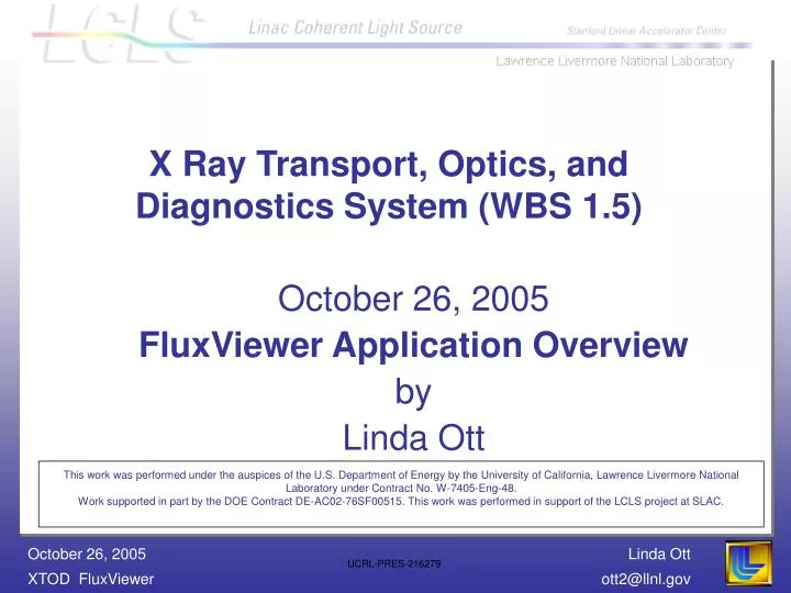
X Ray Transport, Optics, and Diagnostics System (WBS 1.5)

1. X Ray Transport, Optics, and Diagnostics System (WBS 1.5) October 26, 2005 FluxViewer Application Overview by Linda Ott This work was performed under the auspices of the U.S. Department of Energy by the University of California, Lawrence Livermore National Laboratory under Contract No. W-7405-Eng-48.Work supported in part by the DOE Contract DE-AC02-76SF00515. This work was performed in support of the LCLS project at SLAC.

2. Borland Development Environment Borland Supplied GUI Components Forms Edit Boxes Menu Bars … Component Palette Screen Editor Linker Debugger Project Manager Object Inspector Class Explorer Database Engine (BDE) Tools Database Desktop SQL Explorer BDE Administrator … User Supplied LCLS Specific Code Simulation Modeling Data Acquisition Instrument Control Analysis … Third Party Supplied TeeChart Pro Numerical Recipes HDF5 library HDFView Device libraries (eg. Newport ESP6000 Motion Controller PixelVision SDK) Help & Manual InstallShield VisIt LCLS Databases Materials Elements Units Cumlatives ReBin BLOB Objective CCD …

3. Simulations Data Flow Diagram Make Detailed Database Tables GridPointSpectrum CumlativeX,Y,Energy … RawSpontaneous Data Files (UCLA,SLAC) ReBin into Coarser energy bins X Ray Optics Constants Flux Viewer Photon Monte Carlo Applications Add FEL ReBin DB Make BLOB DB Tables Material DB BLOB DBs * Element DB Objective DB Photon Electron Calculator Material DB Attenuator (Gas and Solid) Absorbed, Transmitted, Element DB CCD DB Pixelator (Change Pixel Size) Imager Design Total Energy Monitor Design * Note: BLOB = Binary Large OBjects

4. Raw Spontaneous Data Calculations • Roman Tatchyn (SLAC) • ASCII files • Sven Reiche (UCLA) • HDF5 files

5. Datasets • The dataset files must be downloaded individually • There are 2 file types: All undulator modules (9 datasets) Single undulator module (22 datasets)

6. All Undulator Modules Dir Name EOU (m) Linac E Position S14GeV45 45 14.08 Beginning of Beam Dump S4GeV45 45 4.5 Beginning of Beam Dump S14GeV71 71 14.08 In Beam Dump (“PCPM2”) S4GeV71 71 4.5 In Beam Dump (“PCPM2”) S14GeV83 83 14.08 Beginning of FEE (“MUS1”) S4GeV83 83 4.5 Beginning of FEE (“MUS1”) S14GeV114 114 14.08 End of FEE (“MUS2”) S4GeV114 114 4.5 End of FEE (“MUS2”) S14GeV400 400 14.34 Far Hall Dir Name: Directory name containing the dataset’s database tables EOU (m): Position of simulation from the end of the undulator in meters Linac E: Linac energy in GeV Position: Approximate location of simulation in beam line

7. Approximate Location of Spontaneous Datasets in Beam Line S14GeV71 S4GeV71 (71 m eou) S14GeV400 (400 m eou) S14GeV83 S4GeV83 (83 m eou) S14GeV114 S4GeV114 (114 m eou) S14GeV45 S4GeV45 (45 m eou)

8. Single Undulator Module The single module datasets were were done for two purposes: 1) Determine the camera specifications needed to see undulator radiation from a single segment during commissioning. 14 GeV X Size (1 quadrant) = 60 mm, Y Size = 20 mm Energy resolution = .400 keV, Energy range = 0 to 24,690 keV 4 GeV X Size (1 quadrant) = 200 mm, Y Size = 60 mm Energy resolution = .040 keV, Energy range = 0 to 2,518 keV 2) Decide the practicalities of determining K differences in the undulator segments by measuring the x-ray spectra. X Size (1 quadrant) = 1 mm, Y Size = 1 mm Energy resolution = 1 eV, Energy range = 0 to 30,000 eV

9. Single Undulator Module Folder EOU (m) Linac E Purpose SMFirst4Gev 114 4.36 camera specifications SMFirst14Gev 114 13.64 camera specifications SMLast4Gev 114 4.36 camera specifications SMLast14Gev 114 13.64 camera specifications SMFirstDetuned-3 114 13.64 K study SMFirstDetuned-3_1eVBin 114 13.64 K study SMFirstDetuned-4 114 13.64 K study SMFirstDetuned-4_1eVBin 114 13.64 K study SMFirstNominal 114 13.64 K study SMFirstNominal_1eVBin 114 13.64 K study SMMidDetuned-3 114 13.64 K study SMMidDetuned-3_1eVBin 114 13.64 K study SMMidDetuned-4 114 13.64 K study SMMidDetuned-4_1eVBin 114 13.64 K study SMMidNominal 114 13.64 K study SMMidNominal_1eVBin 114 13.64 K study SMLastDetuned-3 114 13.64 K study SMLastDetuned-3_1eVBin 114 13.64 K study SMLastDetuned-4 114 13.64 K study SMLastDetuned-4_1eVBin 114 13.64 K study SMLastNominal 114 13.64 K study SMLastNominal_1eVBin 114 13.64 K study

10. SpontaneousBlob Database • X Coordinates arrays (lower, center, upper, bin size) • Y Coordinates arrays (lower, center, upper , bin size) • Energy arrays (lower, center, upper , bin size) • Photons array (number photons in each X,Y,Energy bin) • Dataset Parameters: • Position (Distance from End-of-Undulator) • Number of X,Y,Energy bins • Linac Energy (GeV) • Peak Current (A) • Number Undulator Periods • Pulse Duration (seconds) • Undulator K value • Undulator Period (m) • Quadrant Flag (true=1 quad, false=4 quads)

11. Spontaneous Data Chain • UCLA Near-Field Calculator • ~2 Gbyte HDF5 • HDF5 to Paradox Converter • (x,y,E,P) Paradox format, ~7 GByte • ReBinner – Makes Progressively Coarser Energy Bins • (x,y,E,P) Paradox format, 1.2 GByte • Blob DB Converter – faster to read • (E,P[x,y]) Paradox, 160 MBytes • Viewer (FluxViewer)

12. FluxViewer • Spectral flux viewer for BLOB database tables • Allows user to select x,y,energy ranges and display x,y grids, surface plots, energy distributions • Displays #photons, energy (keV, mJ), and fluence (J/cm2) per pulse

13. FluxViewer Help Manual By Richard Bionta Linda Ott Lawrence Livermore National Laboratory October, 2005 UCRL-CODE-216513

14. Application Environment

15. Getting Started…. Select the dataset to view

16. Open Dataset

17. Surface Plot

18. Navigation Click on the Panel Tabs or Speed Buttons to select the panel to be displayed: Change Limits change the query filters Surface Plot 3D plot of the total number of photons in each cell Image Plot 2D plot of the total number of photons in each cell Energy Plot histogram of the photon energies in all cells Fluence 2D Fluence (Joule/cm^2) plot Plot Data tabular list of the data plotted in the surface and image plots DB Display view the dataset database Parameters view parameters used in generating the flux data Export Print/Copy/Save Charts/Data XLineOut histogram of values along x coordinates through selected gridpoint YLineOut histogram of values along y coordinates through selected gridpoint

19. Change Limits

20. Image Plot

21. Energy Distribution in one cell(from click in Image Plot)

22. X, Y LineOuts (from click in Image Plot)

23. Energy Plot Energy distribution for all grid cells. Use the “Change Limits” Panel to define the X,Y,Energy Limits

24. Fluence Plot

25. Surface Plot Data This panel displays the surface and image plot data in tabular form

26. Database Display Displays the data contained in the MasterSpontaneous and SpontaneouBLOB database tables. The Master table contains the bin information for the X and Y Coordinates, and the Energy bins. The BLOB table contains the Number of photons in each X,Y,Energy bin. X coordinates

27. Database Display Select Table to display Energy bins

28. Parameters Displays parameters used to generate the dataset

29. Export Print chart or export charts and data to files or clipboard

30. Export a Chart

31. Export Data

32. X Line Out X and Y LineOuts are created when a user clicks on either an Image Plot or a Fluence Plot

33. Y Line Out The mouse can be used to expand A region. Click and drag to the right to define the Region. Drag mouse left to restore. Zoom In Zoom Out

34. Application and Datasetsare on the LCLS Web Site http://www-ssrl.slac.stanford.edu/lcls/ Project Page Maintenance L2/Dropbox Xray Transport | View# https://www-lcls-internal.slac.stanford.edu/projectspace_L2/xray_transport/ The application is in directory: FluxViewer The datasets are in directory: SpontaneousDBs