Download
1 / 24
240 likes | 313 Views
Goodness of Fit Test. 1. State the null and alternative hypotheses. 2. Select a random sample and record observed frequency f i for the i th category ( k categories ) . Compute expected frequency e i for the i th category:. 4. Compute the value of the test statistic.

E N D
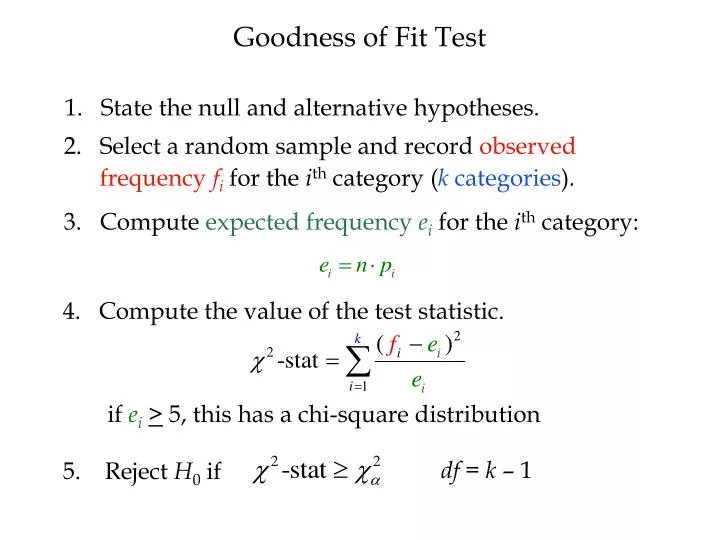
Goodness of Fit Test 1. State the null and alternative hypotheses. 2. Select a random sample and record observed frequency fifor the ith category (k categories). • Compute expected frequency eifor the ith category: 4. Compute the value of the test statistic. if ei> 5, this has a chi-square distribution df = k – 1 5. Reject H0 if
k = 4 Goodness of Fit Test Example: Finger Lakes Homes (A) Finger Lakes Homes manufactures four models of prefabricated homes, a two-story colonial, a log cabin, a split-level, and an A-frame. To help in production planning, management would like to determine if previous customer purchases indicate that there is a preference in the style selected. The number of homes sold of each model for 100 sales over the past two years is shown below. Split- A- Model Colonial Log Level Frame # Sold 30 20 35 15
Goodness of Fit Test ei = (n)(pi) Hypotheses 1/4 .25 H0: pC = pL = pS = pA = Ha: customers prefer a particular style i.e., there is at least one proportion much greater than .25 Expected frequencies e1= (0.25)(100) = 25 e2= (0.25)(100) = 25 e3= (0.25)(100) = 25 e4= (0.25)(100) = 25
Goodness of Fit Test = .05 (column) df = 4 – 1 = 3 (row) Do Not Reject H0 Reject H0 .05 2 m = 3 7.815 At 5% significance, the assumption that there is no home style preferenceis rejected.
Independence Test 1. State the null and alternative hypotheses. 2. Select a random sample and record observed frequency fifor each cell of the contingency table. • Compute expected frequency eij for each cell 4. Compute the test statistic. if ei> 5, this has a chi-square distribution 5. Reject H0 if df = (m - 1)(k - 1)
Independence Test Example: Finger Lakes Homes (B) Each home sold by Finger Lakes Homes can be classified according to price and to style. Finger Lakes’ manager would like to determine if the price of the home and the style of the home are independent variables. The number of homes sold for each model and price for the past two years is shown below. For convenience, the price of the home is listed as either $99,000 or less or more than $99,000. k = 4 m = 2 Price Colonial Log Split-Level A-Frame < $99,000 18 6 19 12 > $99,000 12 14 16 3
Independence Test Observed Frequencies (fi) Price Colonial Log Split-Level A-Frame Total < $99K > $99K Total 18 6 19 12 45 55 12 14 16 3 100 35 15 30 20 Expected Frequencies (ei) Price Colonial Log Split-Level A-Frame Total < $99K > $99K Total 16.5 8.25 11 19.25 55 45 13.5 15.75 9 6.75 30 100 35 20 15
Independence Test Hypotheses H0: Price of the home is independent of the style of the home that is purchased Ha: Price of the home is not independent of the style of the home that is purchased Compute test statistic
Independence Test df = (4 – 1)(2 – 1) = 3 (row) = .05 (column) Do Not Reject H0 Reject H0 .05 2 7.815 m = 3 At 5% significance, we reject the assumption that the price of the home is independent of the style of home that is purchased.
Reject H0 if Goodness of Fit Test: Poisson Distribution 1. Set up the null and alternative hypotheses. 2. Select a random sample and a. Record observed frequencies b. Estimate mean number of occurrences 3. Compute expected frequency of occurrences eifor each value of the Poisson random variable. 4. Compute the value of the test statistic. df = k – p – 1 5.
Goodness of Fit Test: Poisson Distribution Example: Troy Parking Garage In studying the need for an additional entrance to a city parking garage, a consultant has recommended an analysis approach that is applicable only in situations where the number of cars entering during a specified time period follows a Poisson distribution. A random sample of n = 100 one-minute time intervals resulted in the customer arrivals listed below. A statistical test must be conducted to see if the assumption of a Poisson distribution is reasonable. # of Arrivals 0 1 2 3 4 5 6 7 8 9 10 11 12 Frequency 0 1 4 10 14 20 12 12 9 8 6 3 1 otal Arrivals = 0(0) + 1(1) + 2(4) + 3(10) + . . . + 12(1) = 600 Total one-minute intervals = n = 0 + 1 + 4 + 10 + . . . + 1 = 100 Estimate of = 600/100 = 6
Goodness of Fit Test: Poisson Distribution The hypothesized probability of x cars arriving during the time period is For x = 1 0 x f (x ) n∙ f (x ) xf (x ) n∙f (x ) 6 7 8 9 10+ 0 1 2 3 4 5 0.0025 0.1606 0.1377 0.1033 0.0688 16.06 13.77 10.33 6.88 8.39 0.25 1.49 0.0149 4.46 8.92 13.39 16.06 0.0446 0.0892 0.1339 0.1606 0.0839 100.00 1.0000
Goodness of Fit Test: Poisson Distribution ifieifi - ei -1.20 1.08 0.61 3.94 -4.06 -1.77 -1.33 1.12 1.61 5 10 14 20 12 12 9 8 10 0 or 1 or 2 3 4 5 6 7 8 9 10 or more 6.20 8.92 13.39 16.06 16.06 13.77 10.33 6.88 8.39
Goodness of Fit Test: Poisson Distribution With = .05 (column) and df = 7 (row) Do Not Reject H0 Reject H0 .05 2 14.067 At 10% significance, there is no reason to doubt the assumption of a Poisson distribution.
Goodness of Fit Test: Normal Distribution 1. State the null and alternative hypotheses. 2. Select a random sample and a. Compute the mean and standard deviation(p = 2). b. Define intervals so that ei> 5 is in the ith interval c. For each interval, record observed frequencies fi 3. Compute eifor each interval. 4. Compute the value of the test statistic. if ei> 5, this has a chi-square distribution 5. Reject H0 if df = k – p – 1
n = 33, x = 71.76, s = 18.47 Goodness of Fit Test: Normal Distribution Example: IQ Computers IQ Computers (one better than HP?) manufactures and sells a general purpose microcomputer. As part of a study to evaluate sales personnel, management wants to determine, at a 5% significance level, if the annual sales volume (number of units sold by a salesperson) follows a normal probability distribution. A simple random sample of 33 of the salespeople was taken and their numbers of units sold are below. 33 43 44 45 52 52 56 58 63 6364 64 65 66 68 70 72 73 73 74 74 75 83 84 85 86 91 92 94 98 101 102 105
Goodness of Fit Test: Normal Distribution To ensure the test statistic has a chi-square distribution, the normal distribution is divided into kintervals. 6 equal intervals. k = 33/5= 6.6 ei =33/6 =5.5 Expected frequency: The probability of being in each interval is equal to 1/6 = .1667 z.
Goodness of Fit Test: Normal Distribution Find the z that corresponds to the red tail probability = (1)(.1667) = .1667 .1667 z. – .97
Goodness of Fit Test: Normal Distribution Find the z that corresponds to the red tail probability = (2)(.1667) = .3333 .3333 z. –.43
Goodness of Fit Test: Normal Distribution Find the z that corresponds to the red tail probability = (3)(.1667) = .5000 .5000 z. 0
Goodness of Fit Test: Normal Distribution Find the remaining z values using symmetry z. –.97 –.43 0 .43 .97
Goodness of Fit Test: Normal Distribution Find the z that corresponds to the red tail probability Convert the z’s to x’s z. –.97 –.43 0 .43 .97 x
Goodness of Fit Test: Normal Distribution Observed and Expected Frequencies fieifi – ei (fi – ei)2/ei LL UL 0.05 0.41 0.05 0.05 0.41 0.41 1.36 6 5.5 5.5 5.5 5.5 5.5 5.5 33 0.5 -1.5 0.5 0.5 -1.5 1.5 53.84 63.81 71.76 79.70 89.68 ∞ -∞ 53.84 63.81 71.76 79.70 89.68 4 6 6 4 7 33 Total Data Table 33 43 44 45 52 52 56 58 63 6364 64 65 66 68 70 72 73 73 74 74 75 83 84 85 86 91 92 94 98 101 102 105
Goodness of Fit Test: Normal Distribution df = 3 (row) = .05 (column) At 5% significance, there is no reason to doubt the assumption that the population is normally distributed. Do Not Reject H0 Reject H0 .05 2 7.815 m = 3