Download
1 / 59
641 likes | 980 Views
The One-Sample t -Test. Advanced Research Methods in Psychology - lecture - Matthew Rockloff. A brief history of the t-test. Just past the turn of the nineteenth century, a major development in science was fermenting at Guinness Brewery.

E N D
The One-Sample t-Test Advanced Research Methods in Psychology - lecture - Matthew Rockloff
A brief history of the t-test • Just past the turn of the nineteenth century, a major development in science was fermenting at Guinness Brewery. • William Gosset, a brewmaster, had invented a new method for determining how large a sample of persons should be used in the taste-testing of beer. • The result of this finding revolutionized science, and – presumably - beer.
A brief history of the t-test (cont.) • In 1908 Gosset published his findings in the journal Biometrika under the pseudonym ‘student.’ This is why the t-test is often called the ‘student’s t.’
A brief history of the t-test (cont.) Folklore: Two stories circulate for the reason why Gosset failed to use his own name. • 1: Guinness may have wanted to keep their use of the ‘t-test’ secret. By keeping Gosset out of the limelight, they could also protect their secret process from rival brewers. • 2: Gosset was embarrassed to have his name associated with either: a) the liquor industry, or b) mathematics. • But seriously, how could that be?
Thus ??? “Beer is the cause of – and solution to – all of life's problems.” (Homer Simpson)
When to use the one-sample t-test • One of the most difficult aspects of statistics is determining which procedure to use in what situation. • Mostly this is a matter of practice. • There are many different rules of thumb which may be of some help. • In practice, however, the more you understand the meaning behind each of the techniques, the more the choice will become obvious.
Example problem 2.1 • Example illustrates the calculation of the one-sample t-test. • This test is used to compare a list of values to a set standard. • What is this standard? • The standard is any number we choose. • As illustrated next, the standard is usually chosen for its theoretical or practical importance.
Example 2.1 (cont.) • Intelligence tests are constructed such that the average score among adults is 100 points. • In this example, we take a small sample of undergraduate students at Thorndike University (N = 6), and try to determine if the average of intelligence scores for all students at the university is higher than 100. • In simple terms, are the university students smarter than average?
Example 2.1 (cont.) • The scores obtained from the 6 students were as follows: X Person 1: 110 Person 2: 118 Person 3: 110 Person 4: 122 Person 5: 110 Person 6: 150
Example 2.1 (cont.) Research Question On average, do the population of undergraduates at Thorndike University have higher than average intelligence scores (IQ 100)?
= Example 2.1 (cont.) • First, we must compute the mean (or average) of this sample: • In the above example, there is some new mathematical notation. (See next slide)
= Example 2.1 (cont.) • First, a symbol that denotes the mean of all Xs or intelligence scores.
= Example 2.1 (cont.) • The second part of the equation shows how this quantity is computed.
= Example 2.1 (cont.) • The sigma symbol ( ) tells us to sum all the individual Xs.
= Example 2.1 (cont.) • Lastly, we must divide by ‘n’, that is: the number of observations.
= Example 2.1 (cont.) • Notice, these 6 people have higher than average intelligence scores (IQ 100).
Example 2.1 (cont.) • However, is this finding likely to hold true in repeated samples? • What if we drew 6 different people from Thorndike University? • A one-sample t-test will help answer this question. • It will tell us if our findings are ‘significant’, or in other words, likely to be repeated if we took another sample.
Example 2.1 (cont.)Computing the sample variance • To get the third column we take each individual ‘X’ and subtract it from the mean (120). • We square each result to get the fourth column. • Next, we simply add up the entire fourth column and divide by our original sample size (n = 6). • The resulting figure, 201.3, is the sample variance.
Example 2.1 (cont.)Computing the sample variance Important: All sample variances are computed this way! We always take the mean; subtract each score from the mean; square the result; sum the squares; and divide by the sample size (how many numbers, or rows we have).
Example 2.1 (cont.)Computing the sample variance • Now that we have the mean (X = 120) and the variance ( ) of our sample, we have everything needed to compute whether the sample mean is ‘significantly’ above the average intelligence. • In the formula that follows, we use a new symbol mu ( ) to indicate the population standard value ( = 100 ) against which we compare our obtained score (X = 120).
Example 2.1 (cont.)Computing the sample variance Our sample has ‘n = 6’ people, so the degrees of freedom for this t-test are: dn = n – 1 = 5 This degrees of freedom figure will be used later in our test of significance.
And now for something completely different … • Let’s take a break from computations, and talk about ‘the big picture’ Now comes the conceptually tricky part. • Remember that a normal bell-curve distribution is a chart that shows frequencies (or counts). • If we measured the weight of four male adults, for example, we might find the following: • Person 1 = 70 kg, Person 2 = 75 kg, Person 3 = 70 kg, Person 4 = 65 kg
The ‘big picture’ • Person 1 = 70 kg, Person 2 = 75 kg, Person 3 = 70 kg, Person 4 = 65 kg • Plotting a count of these ‘weight’ data, we find a normal distribution: Count 2 X 1 X X X 65 70 75 kg
The ‘big picture’ (cont.) • As it turns out, the ‘t’ statistic has its own distribution, just like any other variable. • Let’s assume, for the moment, that the mean IQ of the population in our example is exactly 100. • If we repeatedly sampled 6 people and calculated a ‘t’ statistic each time, what would we find? • If we did this 4 times, for example, we might find: Count 2 X 1 X X X - 1 0 1 t - statistic
The ‘t’ statistic (cont.) • Most often our computed ‘t’ should be around 0. Why? Because the numerator, or top part of the formula for t is: . • If our first sample of 6 people is truly representative of the population, then our sample mean should also be 100, and therefore our computed t should be (see next slide)
The ‘t’ statistic (cont.) • Of course, our repeated samples of 6 people will not always have exactly the same mean as the population. • Sometimes it will be a little higher, and sometimes a little lower. • The frequency with which we find a t larger than 0 (or smaller than 0) is exactly what the t-distribution is meant to represent (see next slide)
Read this part over and over, and think about it. This is the tricky bit. • In our GPA example, the actual ‘t’ that we calculated was 3.152, which is certainly higher than 0. • Therefore, our sample does not look like it came from a population with a mean of 100. • Again, if our sample did come from this population, we would most often expect a computed ‘t’ of 0
The ‘t’ statistic (cont.) • How do we know when our computed ‘t’ is very large in magnitude? • Fortunately, we can calculate how often a computed sample ‘t’ will be far from the population mean of t = 0 based on knowledge of the distribution.
The ‘t’ statistic (cont.) • The critical values of the t-distribution show exactly how often we should find computed ‘t’s of large magnitude. • In a slight wrinkle, we need the degrees of freedom (df = 5) to help us make this determination. • Why? If we sample only a few people our computed ‘t’s are more likely to be very large, only because they are less representative of the whole population.
And now, back to the computation… • We need to find the ‘critical value’ of our t-test. • Looking in the back of any statistics textbook, you can find a table for critical values of the t-distribution. • Next, we need to determine whether we are conducting a 1-tailed or 2-tailedt-test. • Let’s refer back to the research question:
Example 2.1 (again) Research Question On average, do the population of undergraduates at Thorndike University have higher than average intelligence scores (IQ 100)?
Example 2.1 (cont.) • This is a 1-tailed test, because we are asking if the population mean is ‘greater’ than 100. • If we had only asked whether the intelligence of students were ‘different’ from average (either higher or lower) then the test would be 2-tailed. • In the appendixes of your textbook, look at the table titled, ‘critical values of the t-distribution’. • Under a 1-tailed test with an Alfa-level of and degrees of freedom df = 5, and you should find a critical value (C.V.) of t = 2.02.
Example 2.1 (cont.) Is our computed t = 3.152 greater than the C.V. = 2.02? Yes! Thus we reject the null hypothesisand live happily ever after. Right? Not so fast. What does this really mean?
Example 2.1 (still) • We assume the null hypothesis when making this test. • We assume that the population mean is 100, and therefore we will most often compute a t = 0. • Sometimes the computed ‘t’ might be a bit higher and sometimes a bit lower.
What does the ‘critical value’ tell us? • Based on knowledge of the distribution table we know that 95% of the time, in repeated samples, the computed ‘t’ statistics should be less than 2.02. • That’s what the critical value tells us. • It says that when we are sampling 6 persons from a population with mean intelligence scores of 100, we should rarely compute a ‘t’ higher than 2.02.
What happens if we do calculate a ‘t’ greater than 2.02? • Well, we can be pretty confident that our sample does not come from a population with a mean of 100! • In fact, we can conclude that the population mean intelligence must be higher than 100. • How often will we be wrong in this conclusion? • If we do these t-tests a lot, we’ll be wrong 5% of the time. That’s the Alfa level (or 5%).
Conclusions in APA Style How would we state our conclusions in APA style? The mean intelligence score of undergraduates at Thorndike University (M = 120) was significantly higher than the standard intelligence score (M = 100), t(5) = 3.15, p < .05 (one-tailed).
Statistical inference • You should notice that the conclusion makes an inference about the population of students from Thorndike University based on a small sample. • This is why we call this type of a test ‘statistical inference.’ • We are inferring something about the population based on only a sample of members.
Example 2.1 Using SPSS • First, variables must be setup in the variable view of the SPSS Data Editor as detailed in the previous chapter:
Example 2.1 Using SPSS (cont.) • Next, the data must be entered in the data view of the SPSS Data Editor:
Instructions for the Student Version of SPSS • If you have the student version of SPSS, you must run all procedures from the pull-down menus. • Fortunately, this is easy for the one-sample t-test. • First select the correct procedure from the ‘analyze’ menu see next slide
The ‘test variable’ • Next, you must move the ‘test variable’, in this case IQ, into the right-hand pane by pressing the arrow button and change the ‘test-value’ to 100 (our standard for comparison). • Lastly, click ‘OK’ to view the results:
Instructions for Full Version of SPSS (Syntax Method) • An alternate method for obtaining the same results is available to users of the full-version of SPSS. • This method, known as ‘syntax’, is described here, because many common and useful procedures in statistics are only available using the syntax method. • Users of the student version may wish to skip ahead to ‘Results from the SPSS Viewer.’ • To use syntax, first you must open the syntax window from the ‘file’ menu:
SPSS syntax • The following is generic syntax for the one-sample t-test: • t-test testval=TestValue • /variables=TestVariable. • The SPSS syntax above requires that you substitute two values. • First, you need the ‘TestValue’ against which you are judging your sample. • In example 2.1, this standard is ‘100.’