Download

1 / 36
360 likes | 586 Views
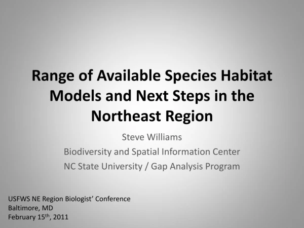
Range of Available Species Habitat Models and Next Steps in the Northeast Region. Steve Williams Biodiversity and Spatial Information Center NC State University / Gap Analysis Program. USFWS NE Region Biologist’ Conference Baltimore, MD February 15 th , 2011. Overview.

E N D
Range of Available Species Habitat Models and Next Steps in the Northeast Region Steve Williams Biodiversity and Spatial Information Center NC State University / Gap Analysis Program USFWS NE Region Biologist’ Conference Baltimore, MD February 15th, 2011
Overview • Model types and tradeoffs • Some pertinent examples • Models being used in Designing Sustainable Landscape projects
Habitat Modeling Approaches • Knowledge Based • dB Matrix • HSI, LSI • Bayesian Belief Network • Statistical Theory • Logistic regression • Occupancy • General linear regression • Poisson Regression • Hierarchical Spatial Count • Time removal • Distance • Machine Learning • Classification & Regression Trees • Random Forests • Artificial Neural Networks • MaxEnt T. Jones-Farrand
Demographic Models (SEPMs) Bioenergetic Models (TRUEMET) Quantitative Models (C&RT) Qualitative Models (HSI) Increasing Strength of Scientific Foundation/Inference Natural History Descriptions Ecological Theory Statistically-sampled Observations Extent of Explanation Process Pattern Data Requirements Large None/Little Cost Large Little Taxon Gamebirds, Endangered Species Waterfowl Shorebirds Landbirds Landbirds T. Jones-Farrand
Population Data Sources • Breeding Bird Survey • Population Info • Index of Relative Abundance (Presence) • Advantages • Consistent protocol & broad spatial coverage • Caveats • Roadside bias • Does not account for detection probability • Poor dataset for some species (e.g. timing, rare habitat) • Testing site-scale relationships T. Jones-Farrand
Population Data Sources • Point Count Surveys (PCD, R8Bird, collect own) • Population Info • Index of Relative Abundance (Presence or Density) • Advantages • Off road, site habitat data, methods to account for detection probability • Testing site-scale relationships • Caveats • Poor temporal & spatial coverage of region • Inconsistent protocols across studies T. Jones-Farrand
Wisdom Knowledge Information Data DIKW Model • Data • Information • Knowledge • Wisdom • Data • Raw observations • 1 black-necked stilt • 3-acre mudflat • MAV • Information • Relevant data given meaning through relational context • 1 black-necked stilt in a 3-acre mudflat in the MAV • Knowledge • A collection of information, whose intent is to be useful • A 3-acre mudflat in the MAV will equal a black-necked stilt • # Stilts = (acresMF)/3 • Wisdom • Synthesis of knowledge and an assessment of its value • Black-necked stilts prefer open habitats with shallow water “No data” means we lack raw observations to feed into statistical modeling techniques It does not mean that we lack understanding or wisdom J. Tirpak
Limitations of Modeling With “No Data” • Expert opinion is subjective • Translation to meaningful population numbers • Rank values • Categorical: marginal, suitable, optimal • Continuous: HSI scores (0.333) • Probabilities • P(0.75) • Expert opinion is subjective • Lack of objectivity • Reflects perspective • Qualitative not quantitative • Relative vs. absolute differences • Communication challenge P (Encounter Site) J. Tirpak
Examples in Practice • HSI models (CHJV & LMVJV) • Bayesian Belief Network (ACJV) J. Tirpak
Overall Habitat Suitability Score Hardwood Basal Area Suitability Score Suitability Score NLCD FIA HSI models (CHJV & LMVJV) J. Tirpak
Bayesian Belief Network - ACJV P (Encounter Site) C.A. Drew
Designing Sustainable Landscapes in the Eastern US • Initial Pilot Area: South Atlantic Migratory Bird Initiative • Future Expansion to Eastern US • SE-GAP data set serves as the base dataset • NE-GAP data set currently underway
Knowledge-Driven Models Utilizing existing GAP models of habitat availability (606 species in SE) Readily available surrogate for relative potential for species occurrence (which are not available) Used in development of Conservation Priority models for each focal species within a habitat guild • SAMBI DSL Species Modeling
SAMBI DSL Species Modeling Data-Driven Models BBS Occupancy probability and range dynamics Test hypotheses about avian range dynamics as function of climate change and other relevant macroecological covariates (e.g., land use change, position within species range, neighborhood effects) – Much stronger inferences than from static habitat-occurrence patterns Provide important response variable – persistence Links alternatives (actions) to fundamental objectives Applicable to limited set of species Useful to validate knowledge-driven models J.A. Collazo
Brown-headed Nuthatchpotential habitat (t00) J.B. Grand
NA LCC Species Modeling • Pilot phase: ~20 species in 3 study areas • Habit@ modeling framework • Multiscale GIS implementation of HSI • Initial models developed by Scott Schwenk (UV) • Predictor variables to include habitat systems & modifiers from the NE Terrestrial Habitat Classification and other ecological settings variables • External peer review • Models implemented by Kevin McGarigal (UMass) • utilizing Settings Spatial dataset containing abiotic, anthropogenic and vegetative derived datalayers
NA LCC Species Modeling • Habit@ - Multi-scale GIS modeling • Local Resource Availability (LRA): the availability of resources important to the species’ life history, such as food, cover, or nesting, at the local, finest scale (a single cell or pixel); • Homerange Capability (HRC): the capability of an area corresponding to an individual’s homerange to support an individual, based on quantity and quality of local resources, configuration of those resources, and condition as determined by intrusions from roads and development; • Population Capability (PC): the capability of an area to not only support a homerange, but its setting in a neighborhood that supports nearby homeranges—that is, the ability of an area to support not only a single individual, but a local population. K. McGarigal
Thanks to contributors: • Todd Jones-Farrand • John Tirpak • Ashton Drew • Barry Grand • Jaime Collazo • Kevin McGarigal • Scott Schwenk
Habit@ Example of Breeding Wood Thrush (draft) Local resource capability for wood thrush is determined separately for the breeding season and post-breeding (pre-migration) season, as follows: S. Schwenk
Habit@ Example of Breeding Wood Thrush (draft) • LRC-B. Local Resource Capability for Breeding • LRB1: Cover [cover1] -- Categorical index; assign weights to each ecological system • LRB2: Canopy closure [closure] -- Continuous logistic function of canopy cover variable. • LRB3: Understory [under] -- Continuous Gaussian function of an index of understory openness. • LRB4: Development intensity 1 [devint1] -- Continuous kernel estimate of development intensity • LRB5: Development intensity 2 [devint2] -- Continuous kernel estimate as above but at a finer scale S. Schwenk
Habit@ Example of Breeding Wood Thrush (draft) • LRC-B. Local Resource Capability for Breeding • LRC-P. Local Resource Capability for Post-Breeding • LRP1: Cover [cover2] -- Continuous linear or logistic function of an index of early successional stage or low vegetation cover. • LRP2: Edge [edge] -- Continuous function of the magnitude of difference in vegetation structure. S. Schwenk
Habit@ Example of Breeding Wood Thrush (draft) • LRC-B. Local Resource Capability for Breeding • LRC-P. Local Resource Capability for Post-Breeding Home range capability for wood thrush is determined separately for the breeding season and post-breeding (pre-migration) season, as follows; S. Schwenk
Habit@ Example of Breeding Wood Thrush (draft) • LRC-B. Local Resource Capability for Breeding • LRC-P. Local Resource Capability for Post-Breeding • HRC-B. Home Range Capability for Breeding • HRB1: Kernel [bkernel] -- For each focal cell with LRC-B>0, build a resistant kernel scaled to home range size with resistance weights derived from a variable such as vegetation biomass or canopy height that effectively provides low resistance to increasingly mature forest and high resistance to non-forest and development, and then compute the kernel-weighted sum of the LRC-B values and return the value to the focal cell. Note, here we build resistant kernel home ranges only for cells that confer breeding habitat value. S. Schwenk
Habit@ Example of Breeding Wood Thrush (draft) • LRC-B. Local Resource Capability for Breeding • LRC-P. Local Resource Capability for Post-Breeding • HRC-B. Home Range Capability for Breeding • HRC-P. Home Range Capability for Post-Breeding • HRP1: Kernel [pkernel] -- Computed to take into effect the distance moved from from breeding season range to post-breeding season range. S. Schwenk
Habit@ Example of Breeding Wood Thrush (draft) • LRC-B. Local Resource Capability for Breeding • LRC-P. Local Resource Capability for Post-Breeding • HRC-B. Home Range Capability for Breeding • HRC-P. Home Range Capability for Post-Breeding Home range capability is computed as the product of HRC-B and HRC-P. S. Schwenk
GAP National Environmental Spatial Data • GAP National Land Cover Data • Ecological systems • Elevation • Slope • Aspect • Forest/nonforest edge • Forest interior • Percent canopy cover • Hydrography • Proximity to water features • Stream velocity • Human impacts (road & urban density)
Contributions from Gap Analysis Program • Continental extent • WHR dB based on Ecological Systems • Hierarchical approach to species modeling • Known Range – all species • Predicted Distribution – all species • Habitat Importance – subset of species
Contributions from Gap Analysis Program • Continental extent • WHR dB based on Ecological Systems • Hierarchical approach to species modeling • Bayesian framework for model development • Bayesian Belief Network via Elicitator • Integrated with ArcGIS and R to provide immediate feedback • Measures of uncertainty due to system variability and expert diversity and confidence James et al (2009) Elicitator : an expert elicitation tool for regression in ecology. Environmental Modelling & Software, 25(1), pp. 129-145.
National GAP Wildlife Habitat Relationship (WHR) Database • Built upon recent regional GAP databases • 2011 spp. of terrestrial vertebrates in lower 48 317 Complete / 1078 Partial / 616 Undone • 3,267 individual models either draft or final (by season, by region) • Prioritizing birds, NE SGCN species, reptiles
SAMBI DSL Priority model Combine densities to map priority for each species Limiting factors (*) Suitable longleaf sites (S) Potential to use fire (F) Compensatory factors (+) Putative source populations (P)1 Public lands (L) Distance to potential habitat (H)11Species specific data Priority = S*F*(P+L+H) J.B. Grand
Suitability (t00) J.B. Grand
Fire potential(t00) J.B. Grand
Conservation Lands(t00) J.B. Grand
Priority for Brown-headednuthatch for t00 Priority = suitability * burnability * (potential habitat + conservation lands + source populations) J.B. Grand