Download
1 / 15
150 likes | 266 Views
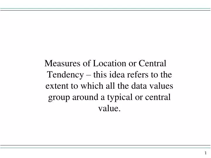
Measures of Location or Central Tendency – this idea refers to the extent to which all the data values group around a typical or central value. Section overview.

E N D
Measures of Location or Central Tendency – this idea refers to the extent to which all the data values group around a typical or central value.
Section overview In this section we will look at the statistical tools called measures of location or central tendency. The basic idea is that we are trying to find the “middle” response or value on a variable. The three measures we explore in this section are the mode, median, and mean. Silly analogy: In many sports, a defensive player guards an offensive player. Offensive players can be crafty. They might use their eyes to indicate where they might go, but then they go another way. With their eyes they have tricked the defense to think their location will be one place and then they go another. Coaches have picked up on this and they say do not follow the eyes, follow the center, or gut, of the player. “The center will tell you about location.” I can still hear my coach say this. He also said, “Parker, not only are you short, you are slow too.”
The Mode When you have a variable you can look at each of the responses the subjects have put. Some subjects have put the same response. The response that has been put most frequently is called the mode. Remember we said variables can be categorical or numerical. The mode can be used on any type of variable in terms of level of measurement. But, the mode is probably used most when the variable is categorical. When you have a frequency distribution, the mode can be reported as an additional description about the distribution.
The Mode How can you find the mode? The frequency distribution in counts will show the VALUE with the most counts. Sometimes a variable will have a tie for the mode. In this case two or more VALUES will have the same, and most, counts. The variable in then said to be multimodal.
The Median Let’s think of a simple data set, say, the height of the 5 people in a family: (all in feet - actually shoes, but measured in feet) 5.6, 6.6, 5.33, 6.0 and 5.0. Now let’s order or sort the numbers from low to high - sometimes called increasing or ascending order: 5.0, 5.33, 5.6, 6.0, and 6.6. Here we have 5 numbers. In general we say the data set is of size n. Here n = 5. The 3rd number, in the sorted data set, or in general the number in the (n+1)/2 position in the order, is called the median. The median here is 5.6 Note here n is an odd number (n = 5). What if n is even?
The Median Let’s think of another simple data set, say, the height of the 4 people in a family: 5.6, 6.6, 5.33, and 6.0. Now let’s order or sort the numbers from low to high - 5.33, 5.6, 6.0, and 6.6. Here we have 4 numbers, or n = 4. If we take (n+1)/2 we get (4+1)/2 = 2.5. But wait, we have the 1st, 2nd, 3rd and 4th numbers, not the 2.5th number. But 2.5 falls between the 2nd and 3rd number in order. The median of the data is the average of the values in the 2nd and 3rd order - here the median is 5.8 feet. How did I get 5.8?
The Median • Note the way the median is found • arrange or sort the data in increasing order • n is the number of data points • If n is odd, the data point or value in the (n+1)/2 spot, starting with the lowest, is the median • If n is even, (n+1)/2 has the decimal • .5 and the median is the average of the data points • on each side of the .5 number. • The median is a measure of center because after the data • is sorted the median is the value where half the data are • less and half the data are more than the median. The median is also known as the 50th percentile.
The Mean Let’s do a simple example to see why the mean is a measure of center. What is the mean of the following 4 numbers: 5, 6, 7, 8? x (read as xbar for mean) = (5 + 6 + 7 + 8)/4 = 6.5 5 6 7 8 On the next screen we will look at the distance of each number from the mean by taking the number minus the mean. This value is called a deviation.
The Mean The data points The points minus the mean 5 5 - 6.5 (= - 1.5) 6 6 - 6.5 (= - .5) 7 7 - 6.5 (= .5) 8 8 - 6.5 (= 1.5) Note the column of deviations adds up to zero. Points to the right of the mean (numbers 7, 8) are a positive distance and points to the left are a negative distance. The mean is a measure of center because the positive and negative distances cancel out to zero.
Compare Parker’s example: Compare the two data sets below by computing the mean and median for each. set A: 1, 2, 3 set B: 1, 2, 99 mean=................. mean=.................. median=............... median=.............. Note how the median resists changing value in the presence of an extreme value in set B (the mode has this property as well). The median is often used in studies where extreme observations occur. Studies of income data typically have median reported as the measure of center.
Analysis I have drawn here a frequency distribution and I have put on top of it a bell shaped curve. In many cases when you can put a bell shaped curve on the frequency distribution the distribution is called normal.
Normal Distribution In a normal distribution there is one mode - a unimodal distribution, the distribution is symmetric - from the center, the left and the right are mirror images of each other (the tails are the same), the mean = median,
Populations and Samples At this time I want you think about the difference between a sample and population. In fact, let’s think about the population of Wayne, America. There are about 5,400 people who live in Wayne. Say we do a census in Wayne and obtain the age of everyone in Wayne. In this case the mean would be called a population parameter. A parameter is just a key, or important, feature of a population. If we just did a sample of residents in Wayne and talked to 200 people we could get the sample mean. The sample mean is an example of a sample statistic. A statistic is a key feature of a sample.
In a class such as ours we use symbols or letters to represent things for us in a shorthand notation. Let’s consider some shorthand when we consider a population. N = the total number of people (or what ever the subjects consist of) in the population. μ = the population mean, spelled mu, which rhymes with new, but not when the cow says moo. I hate to be a word snob, but when someone says moo, for mu, then I know they are uninformed or careless with their language. Σ means add up, or take the sum. Xi is a way to say the ith person has the value X on the variable. μ = Σ Xi / N - the population mean is the sum of all the values on the variable divided by the size of the population.
Now let’s consider some shorthand when we consider a sample. n = the total number of people in the sample. x = the sample mean, called x bar. Σ means add up, or take the sum. xi is a way to say the ith person has the value x on the variable. x = Σ xi / n or the sample mean, is the sum of the values on the variable in the sample divided by the size of the sample. Foreshadowing of things to come: when we do not know the population parameter and when a sample from the population is obtained, the sample statistic can be used as a point estimator of the population parameter. A point estimator is a method used to make an “educated guess” about the value of an unknown population parameter.