Download

1 / 29
290 likes | 373 Views
Development of the Finnish labour market. Annual Meeting of the International Forecasting Network Helsinki May 9/10 2011 Ilkka Nio. Finland has got rid of the global recession.

E N D
Development of the Finnish labour market Annual Meeting of the International Forecasting Network Helsinki May 9/10 2011 Ilkka Nio
Finland has got rid of the global recession • In 2009 the GDP decreased in 2009 by 7.2 % but quite rapid growth started from the second half of 2010. Growth for the year 2010 was 3.1 per cent. All demand items are contributing positively to growth, with exports as the strongest driver. • Earnings increased rapidly in 2009 relative to the cyclical environment keeping up the positive expectations and private consumption, which started grow during the last quarter of 2009. In 2010 it grew by 2 %. However, many facts indicate only modest growth of consumption. The new wage settlements will likely be rather moderate after the recession.Purchasing power will be eroded by rising interest rates and the acceleration of inflation. • Negative risks are associated with the public sector indebtedness and financial imbalances and the slow pace of employment growth. Finland's strong public finances deteriorated sharply during the economic crisis, although the deficit is still under the 3 % threshold. • Economic growth forecast for 2011-2013 is not high enough that the deficit in state finances would turn into a surplus during the economic recovery, but without additional measures, they will continue to remain in deficit in 2015. • All in all, the Finnish economy is expected to grow by 4 % in 2011. Without Nokia´s production problem the GDP would increase even more. The growth is expected to continue moderately ( 2-3 %) during the next years.
Supply and demand of labour • Alongside the growth of the economy the demand for labour has started to strengthen slowly. • Young peolple were mainly influenced by the impacts of the recession, while the aged labour force kept their jobs and stayed in the labour market. It seems that working careers are still being prolonged. • Even then the changing population age structure will begin to affect the supply of labour. The ageing of the population will soon begin to constrain the labour market. • The number of hours worked by persons employed fell during the recession twice as much as the number of people in employment: the number of hours worked dropped by 6 % and the number of persons employed only by 3 %. • Employment is expected to grow slowly. In particular the financial problems of the public sector will limit employment opportunities. The productivity will be raised by rationalizing the use of current labour force. Employment will start to grow faster after the labour input and production are rebalanced.
Expectation of time spent in the labour market at age 50 in 1990 - 2010
Unemployment situation • The deterioration of labour market situation during the crisis was not as bad as predicted. Companies were keen to retain their skilled staff, offering them shorter working hours and layoffs over redundancies. (Labour hoarding) • Part of the reason behind the recent decreasing unemployment is the considerable increase in the use of active labour market policy measures. • The structural composition of unemployment has been aggravated. The long-term unemployment and structural unemployment has increased, slowing down the decrease of total unemployment. • The unemployment rate ( 8.4 % in 2010) will decrease annually by not more than one percentage point > to 7,5 per cent in 2011 and on to 6,5 per cent in 2012.
Unemployment rates according to the LFS and JSR in 1989 - 2011 (III)
Youth unemployment according to the jobseekers register and Labour Force Survey 1991 – 2011 (III)
Hysteresis or persistence in Unemployment ? • There is considerable evidence ( micro and macro ) that hysteresis ( or persistence) of unemployment is an important factor in the Finnish labour market. • Strong negative duration dependence means rapidly declining chances of becoming employed when the duration of unemployment spell lengthens. • Persistent high unemployment can lead to an increase in the long-term natural rate of unemployment ( NAIRU) determined in the labour market.Different country can follow different time path in achieving the equilibrium. • The effects of shocks are difficult to assess and forecast. Hysteresis is a lagging variable among explanatory variables of unemployment. • Overcoming the problem of hysteresis has been the major policy issue in Finland. For this purpose a specific indicator was created in 2003 to measure the core of structural unemployment. In March it accounted for 144 000 ( 5,5 % ). • Considerable increase in the use of ALMP measure ( in March 4,1 %)
Unemployed persons seeking work (1) and unfilled vacancies at the employment service (2) . Original monthly figures and seasonally adjusted figures (S)
Average duration of incomplete unemployment ( stock) is a lagging cyclical indicator
Unemployed and persons placed on ALMP-measures, per cent of labour force 1988-2011( III)
Both quantitative and qualitative methods are used in order to get maximum information from the available data Big macroeconomic models do not provide robust information to forecast the turning points and cyclical changes in employment. >> Need for short term forecasts. Qualitative approach • Collecting qualitative information from regions • Comparing the forecasts of different authors • Herd instinct among forecasters > The forecasts do not often differ much from each others Time Series Analysis ( STAMP, ARIMA) • Monthly follow up of time series from the economy and the labour market • Specification of cyclical, seasonal and irregular variations in order to search turning points Experimental quantitative approach • Often simple models are useful to help understanding the relationships between the economy and the labour market. • Searching leading indicators • It is difficult to interprete the variables regarding expectations
Expectations, one year ahead by regions Unemployment rate by regions 2010 Spring 2011 Whole country 8.4 % 11,0 % and more 9,0 % - 10,9 % 7,0 % - 8,9 % Less than 7,0 % Lappi Lappi 11,3 Little decline Very little decline No change Pohjois- Pohjanmaa Pohjois- Pohjanmaa Kainuu 10,2 Kainuu Source: MEE Source: Statistics Finland 9,0 Pohjois- Savo Pohjois- Savo Pohjois- Karjala Pohjois- Karjala Etelä- Pohjanmaa Etelä- Pohjanmaa Pohjanmaa Pohjanmaa 10,0 Keski- Suomi 12,5 Keski- Suomi 6,7 8,2 Etelä-Savo Pirkan- maa Etelä-Savo 9,9 Pirkan- maa 7,9 Satakunta Satakunta Häme 9,7 8,8 Kaakkois-Suomi Häme Kaakkois-Suomi 9,0 10,6 Varsinais-Suomi Varsinais-Suomi Uusimaa Uusimaa 8,1 6,4
STAMP Structural Time Series Analyser, Modeller and Predictor • Follow up of estimated local trends every month in order to understand the behaviour of the time series and the fit of the forecasts. • Labour market figures are dominated by stochastic trend component • without explanatory variables forecasting possible only in the very short run • The aim of structural time series modelling is the specification of various components: cyclical, seasonal and irregular. The components are considered as stochastic unobserved components which are assessed by looking at the behaviour of the series throughout the whole sample rather than at the end of the period. • Comparing the structural time series models with ARIMA models, the essential difference is that the trend or the unit root component is modelled together with the stationary part of time series. There are two parts to the trend: Stochastic level which is the actual value of the trend and stochastic slope. • Kalman filter forecasts the continuation of the series and also gives, as a side product, the estimates for the unobserved components. The forecast function of STAMP estimation is a straight line with upward or downward slope. • Including explanatory variables in a structural time series model - as stochastic variables - results in a mixture of time series and classical regression. • The combination of unobserved stochastic components with explanatory variables opens in principle many possibilities for dynamic modelling. However, in practice the choice of potential explaining variables is rather limited. • The predictive power of forecasts can be strengthened by means of leading economic indicators such as business expectations or business assessment using data on order books, various confidence indexes, stock market index, etc
Consumers´ confidence ( saldo) and change in employment ( slope), 1000 persons, monthly figures ( 2011 III)
Consumers´ confidence ( saldo) and change in unemployment ( slope 1000 persons), monthly figures until 2011 (III)
Cross-correlation of consumers´ confidence and slope of unemployment, monthly figures
Quantitative experimental approach • Purpose is to find handy and simple models which could be precise, convincing and clear enough, so as to be interesting for decision-makers • Starting with simple models which contain just a small number of equations and variables formulated on a priori considerations, in order to combine the theoretical considerations with the empirical observations. • Different calculations are carried out by adding explanatory variables in various combinations and taking advantage of background economic forecasts for output and various demand items, which have a lead over the employment data. Changing their values, the path of the forecasts can be examined under different scenarios. • Due to intercorrelated variables, we need to compromise with the scientific needs regarding explanatory ability and accuracy of the estimates ( when certain that the same pattern of multicollinearity of dependent variables will continue ). • However, there is no standard business cycle and thus the stability of the estimates and their sensitivity to the changes in the sample period can vary.
Model: Dependent variable: Quarterly change in employment Explanatory variables: change in demand items, lag 2 quarters Method: Least squares, R-squared 0,69
Fit of employment model, 1000 persons, demand items as explanatory variables