Download
1 / 41
410 likes | 501 Views
Climate Models and Their Evaluation, Part 2. Reminder: What is a Model?. Substitute for reality Closely mimics some essential elements Omits or poorly mimics non-essential elements. Reminder: What is a Model?.

E N D
Reminder: What is a Model? • Substitute for reality • Closely mimics some essential elements • Omits or poorly mimics non-essential elements
Reminder: What is a Model? • Quantitative and/or qualitative representation of natural processes (may be physical or mathematical) • Based on theory • Suitable for testing “What if…?” hypotheses • Capable of making predictions
What is a Model? Input Data Model Output Data What input data might we consider for a typical climate model? What output data might we consider for a typical climate model? Tunable Parameters What are the tunable parameters of interest?
S, , a, g, Ω O3 H2O CO2 Ω CLIMATE DYNAMICS OF THE PLANET EARTH g a (albedo) Gases: H2O, CO2, O3 S T4 h*: mountains, oceans (SST) w*: forest, desert (soil wetness) CLIMATE . stationary waves (Q, h*), monsoons WEATHER hydrodynamic instabilities of shear flows; stratification & rotation; moist thermodynamics day-to-day weather fluctuations; wavelike motions: wavelength, period, amplitude
What is Model Evaluation? • Validation • Confirmation that formulation of model conforms to intent (equations, algorithms, units, specified parameters etc.) • Confirmation that outputs are, within tolerable limits, as expected for given inputs • Verification • Comparison with known, measured (observed) quantities • Means, variability (frequency, amplitude, phase) • Spatial structure (scale, shape, amplitude) • Simulation: confirms theory for specified circumstances (e.g. specified boundary conditions) • Prediction: accurately reproduces time series of observed evolution from specified initial conditions • (Inter-)Comparison • Comparison among different models’ outputs for identical inputs
Evaluating the IPCC Models • Important question: What do climate models have to be able to do in order to • Provide quantitative/probabilistic, accurate, reliable, and useful (for adaptation or mitigation) estimates of future climate conditions • Establish the cause of a given aspect of climate change, e.g., its possible anthropogenic origin
SST (1980-1999) SAT (1961-1990) Figure 8.2 OBS (contours) & mean MME error (shades) MME RMS error
SST & SAT st. dev. Figure 8.3 OBS (contours) & mean MME error (shades)
RMS error w.r.t. ERBE mean error in SWTOA mean error in OLR
Annual Mean Precipitation 1980-1999 OBS MME
Climate Model Fidelity and Projections of Climate Change J. Shukla, T. DelSole, M. Fennessy, J. Kinter and D. Paolino Geophys. Research Letters, 33, doi10.1029/2005GL025579, 2006
Annual Mean, Zonal Mean Oceanic Heat Transport Figure 8.6
Annual Mean, Zonal Mean ZonalSfc Wind Stress (Nm-2) Figure 8.7
Annual Mean, Zonal Mean SST Error Figure 8.8
Figure 8.11 Figure 8.11. Normalized RMS error in simulation of climatological patterns of monthly precipitation, mean sea level pressure and surface air temperature. Recent AOGCMs (circa 2005) are compared to their predecessors (circa 2000 and earlier). Models are categorized based on whether or not any flux adjustments were applied.
scaling by reference ensemble average over all variables Reichler and Kim, 2008 (BAMS)
Flux-adjusted Flux-adjusted Non-flux-adjusted Reichler and Kim, 2008 (BAMS)
Deseasonalized changes in precipitation (mm/day) for observations and AMIP3 models for the tropics. Gray shading denotes the model ensemble mean ±1 standard deviation. Also shown in Figure 1b is -0.1 * Multivariate ENSO Index (MEI) [Allan and Soden, 2007]
Upper 700m (complete) Volume-Averaged Ocean Temperature Upper 700m (sub-sample) Upper 3000m (complete) Simulated and observed changes in volume-averaged temperature of the top 700 m (A and B) and 3,000 m (C and D) of the global ocean. Model results are from simulations of 20th century climate change performed with two atmosphere/ocean general circulation models: MIROC3.2 (medres) and CGCM3.1 (T47). Observations are from the WOA-2005 data set and the ISHII6.2 data set. The ISHII6.2 data are available for 0 –700 m only. Results are shown for both spatially complete temperatures (A and C) and temperatures subsampled with the WOA-2005 coverage mask (B and D). The multimodel V and No-V ensemble means are also plotted. These are based on 28 (16) realizations of the 20c3m experiment that included (excluded) volcanic forcing. Control run drift was removed from the model results. (Achuta-Rao et al. 2007) Upper 3000m (sub-sample)
Amplitude (mm) of annual cycle of land water storage from GRACE and 5 climate models. [Swenson & Milly, 2006]
Zonal Mean Ocean Potential Temperature (1957-1990) Figure 8.9 OBS (WOA - Levitus 1957-1990; contours) & mean MME error (shades) Figure 8.9. Time-mean observed potential temperature, zonally averaged over all ocean basins (labeled contours) and multi-model mean error in this field, simulated minus observed (color-filled contours).
Sea Ice Distribution (1980-1999) Figure 8.10 > 15% concentration OBS - red line March September Figure 8.10. Baseline climate (1980–1999) sea ice distribution simulated by 14 of the AOGCMs for March (left) and September (right), adapted from Arzel et al. (2006). For each 2.5x 2.5 longitude-latitude grid cell, the figure indicates the number of models that simulate at least 15% of the area covered by sea ice. The observed 15% concentration boundaries (red line) are based on HadISST.
Summer SH SLP EOF1 (1950-1999) Figure 8.12 Figure 8.12. Ensemble mean leading EOF of summer (Nov-Feb) Southern Hemisphere SLP for 1950 to 1999. The EOFs are scaled so that the associated PC has unit variance over this period. The percentage of variance accounted for by the leading mode is listed at the upper left corner of each panel. The spatial correlation (r) with the observed pattern is given at the upper right corner. At the lower right is the ratio of the EOF spatial variance to the observed value.
NINO3 Surface Air Temperature spectra (MEM; 1980-1999) Figure 8.13 CMIP3 (AR4) CMIP2
Figure 8.14 water vapor clouds albedo long-wave radiation
Figure 8.15 ascending descending The discrepancy between the two groups of models is greatest in regimes of large-scale subsidence. These regimes, which have a large statistical weight in the tropics, are primarily covered by boundary-layer clouds. As a result, the spread of tropical cloud feedbacks among the models (inset) primarily arises from inter-model differences in the radiative response of low-level clouds in regimes of large-scale subsidence.
The climate change s/Ts values are the reduction in springtime surface albedo averaged over Northern Hemisphere continents between the 20th and 22nd centuries divided by the increase in surface air temperature in the region over the same time period. Seasonal cycle s/Ts values are the difference between 20th-century mean April and May as averaged over Northern Hemisphere continents divided by the difference between April and May Ts averaged over the same area and time period.
FAQ 8.1, Figure 1 OBS MME Global Mean Surface Air Temperature (anomaly w.r.t. 1901-1950 mean)
Zonal Mean Surface Air Temperature & Precipitation from EMICs @ c(CO2) = 280 ppm Figure 8.17 + OBS + OBS O OBS O OBS