Download
1 / 40
411 likes | 645 Views
Edge Preserving Image Restoration using L 1 norm. Vivek Agarwal The University of Tennessee, Knoxville. Outline. Introduction Regularization based image restoration L 2 norm regularization L 1 norm regularization Tikhonov regularization Total Variation regularization

E N D
Edge Preserving Image Restoration using L1 norm Vivek Agarwal The University of Tennessee, Knoxville
Outline • Introduction • Regularization based image restoration • L2 norm regularization • L1 norm regularization • Tikhonov regularization • Total Variation regularization • Least Absolute Shrinkage and Selection Operator (LASSO) • Results • Conclusion and future work
Introduction -Physics of Image formation Imaging system g(x,y) K(x,y,x’,y’) f(x’,y’) Registration system g(x,y)+noise noise Reverse Process Forward Process
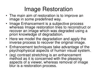
Image Restoration • Image restoration is a subset of image processing. • It is a highly ill-posed problem. • Most of the image restoration algorithms uses least squares. • L2 norm based algorithms produces smooth restoration which is inaccurate if the image consists of edges. • L1 norm algorithms preserves the edge information in the restored images. But the algorithms are slow.
Well-Posed Problem In 1923, the French mathematician Hadamard introduced the notion of well-posed problems. According to Hadamard a problem is called well-posed if • A solution for the problem exists (existence). • This solution is unique (uniqueness). • This unique solution is stable under small perturbations in the data, in other words small perturbations in the data should cause small perturbations in the solution (stability). If at least one of these conditions fails the problem is called ill or incorrectly posed and demands a special consideration.
Existence To deal with non-existence we have to enlarge the domain where the solution is sought. Example: A quadratic equation ax2 + bx +c =0 in general form has two solutions: There is a solution Real Domain No SolSution Complex domain Non-existence is Harmfull
Uniqueness Non-uniqueness is usually caused by the lack or absence of information about underlying model. Example: Neural networks. Error surface has multiple local minima and many of these minima fit training data very well, however Generalization capabilities of these different solution (predictive models) can be very different, ranging from poor to excellent. How to pick up a model which is going to generalize well? Solution #3 Bad or good? Solution #1 Bad or good? Solution #2 Bad or good?
Uniqueness • Non-uniqueness is not always harmful. It depends on what we are looking for. If we are looking for a desired effect, that is we know how the good solution looks like then we can be happy with multiple solutions just picking up a good one from a variety of solution. • The non-uniqueness is harmful if we are looking for an observed effect, that is we do not know how good solution looks like. • The best way to combat non-uniqueness is just specify a model using prior knowledge of the domain or at least restrict the space where the desired model is searched.
Instability Instability is caused by an attempt to reverse cause-effect relationships. Nature always solves just for forward problem, because of the arrow of time. Cause always goes before effect. In practice very often we have to reverse the relationships, that is to go from effect to cause. Example: Convolution-deconvolution, Fredhold integral equations of the first kind. Forward Operation Effect Cause
L1 and L2 Norms The general expression for norm is given as L2 norm: is the Euclidean distance or vector distance. L1 norm: is also known as Manhattan norm because it corresponds to the sum of the distances along the coordinate axes.
Why Regularization? • Most of the restoration is based on Least Squares. But if the problem is ill-posed then least squares method fails.
Regularization The general formulation for regularization techniques is Where is the Error term is the regularization parameter is the penalty term
Tikhonov Regularization • Tikhonov is a L2 norm or classical regularization technique. • Tikhonov regularization technique produces smoothing effect on the restored image. • In zero order Tikhonov regularization, the regularization operator (L) is identity matrix. • The expression that can be used to compute, Tikhonov regularization is • In Higher order Tikhonov, L is either first order or second order differentiation matrix.
Tikhonov Regularization Original Image Blurred Image
Total Variation • Total Variation is a deterministic approach. • This regularization method preserve the edge information in the restored images. • TV regularization penalty function obeys the L1 norm. • The mathematical expression for TV regularization is given as
Difference between Tikhonov regularization and Total Variation
Computation Challenges Total Variation Gradient Non-Linear PDE
Computation Challenges (Contd..) • Iterative method is necessary to solve. • TV function is non-differential at zero. • The is non-linear operator. • The ill conditioning of the operator causes numerical difficulties. • Good Preconditioning is required.
Computation of Regularization Operator Total Variation is computed using the formulation. The total variation is obtained after minimization of the Least Square Solution Total Variation Penalty function (L)
Computation of Regularization Operator Discretization of Total variation function: Gradient of Total Variation is given by
Regularization Operator The regularization operator is computer using the expression Where
Lasso Regression • Lasso for “Least Absolute Shrinkage and Selection Operator” is a shrinkage and selection method for linear regression introduced by Tibshirani 1995. • It minimizes the usual sum of squared errors, with a bound on the sum of the absolute values of the coefficients. • The computation of solution for Lasso is a quadratic programming problem that can be best solved by least angle regression algorithm. • Lasso also uses L1 penalty norm.
Ridge Regression and Lasso Equivalence • The cost function of ridge regression is given as • Ridge regression is identical to Zero Order Tikhonov regularization • Analytical Solution of Ridge and Tikhonov are similar • The bias introduced favors solution with small weights and the effect is to smooth the output function.
Ridge Regression and Lasso Equivalence • Instead of single value of λ,different values of λ can be used for different pixels. • It should provide same solution as lasso regression (regularization). • Thus we establish relation between lasso and Zero Order Tikhonov, there is a relation between Total Variation and Lasso Tikhonov Our Aim To Prove Proved Total Variation Lasso Both are L1 Norm penalties
L1 norm regularization - Restoration Synthetic Images Input Image Blurred and Noisy Image
L1 norm regularization - Restoration Total Variation Restoration LASSO Restoration
L1 norm regularization - Restoration I Deg of Blur II Deg of Blur III Deg of Blur Blurred and Noisy Images Total Variation Regularization LASSO Regularization
L1 norm regularization - Restoration I level of Noise II level of Noise III level of Noise Blurred and Noisy Images Total Variation Regularization LASSO Regularization
Cross Section of Restoration Different degrees Of Blurring Total Variation Regularization LASSO Regularization
Cross Section of Restoration Different levels of Noise Total Variation Regularization LASSO Regularization
Comparison of Algorithms Original Image LASSO Restoration Tikhonov Restoration Total Variation Restoration
Effect of Different Levels of Noise and Blurring LASSO Restoration Blurred and Noisy Image Tikhonov Restoration Total Variation Restoration
Numerical Analysis of Results - Airplane First Level of Noise Second Level of Noise
Graphical Representation – 5 Real Images Different degrees of Blur Restoration Time Residual Error
Graphical Representation - 5 Real Images Different levels of Noise Restoration Time Residual Error
Conclusion • Total variation method preserves the edge information in the restored image. • Restoration time in Total Variation regularization is high • LASSO provides an impressive alternative to TV regularization • Restoration time of LASSO regularization is two times less than restoration time of RV regularization • Restoration quality of LASSO is better or equal to the restoration quality of TV regularization
Conclusion • Both LASSO and TV regularization fails to suppress the noise in the restored images. • Analysis shows increase in degree of blur increases the restoration error • Increase in the noise level does not have a significant influence on the restoration time but effects the residual error