Download
1 / 9
90 likes | 96 Views
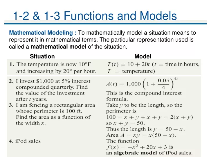
1- 2 & 1-3 Functions and Models. Mathematical Modeling : To mathematically model a situation means to represent it in mathematical terms. The particular representation used is called a mathematical model of the situation . Situation Model.

E N D
1-2 & 1-3 Functions and Models Mathematical Modeling : To mathematically model a situation means to represent it in mathematical terms. The particular representation used is called a mathematical model of the situation. Situation Model
COST – REVENUE – PROFIT MODELSExample – Modeling Cost: Cost Function • As of October 2007, Yellow Cab Chicago’s rates were $1.90 on entering the cab plus $1.60 for each mile. • a. Find the cost C of an x-mile trip. • b. Use your answer to calculate the cost of a 40-mile trip. • c. What is the cost of the 2nd mile? What is the cost of the 10th mile? • d. Graph C as a function of x. A) C(x) = 1.60x + 1.90 (Variable Cost: 1.60x Fixed Cost: 1.90) Cost = Variable Cost + Fixed Cost. Marginal Cost: The incremental cost per mile - 1.60 (slope) B) Cost of a 40 mile trip: C(40) = 1.60(40) + 1.90 = $65.90 C) Cost of 2nd Mile = C(2) – C(1) = $1.60 (cost of each additional mile)
Cost, Revenue, and Profit Models • Cost, Revenue, and Profit Functions • A cost function specifies the cost C as a function of the number of items x. Thus, C(x) is the cost of x items, and has the form • Cost = Variable cost + Fixed cost => C(x) = mx + b • (m = marginal cost b = fixed cost) • If R(x) is the revenue (gross proceeds) from selling x items at a price of m each, then R is the linear function R(x) = mx and the selling price m can also be called the marginal revenue. • The profit (net proceeds) is what remains of the revenue when costs are subtracted. Profit = Revenue – Cost (Negative profit is Loss)
Cost, Revenue, and Profit Models • Break Even: Neither Profit nor Loss. Profit = 0 & C(x)=R(x) • The break-even point : the number of items x at which break even occurs. • Example • If the daily cost (including operating costs) of manufacturing x T-shirts is C(x) = 8x + 100, and the revenue obtained by selling x T-shirts is R(x) = 10x, then the daily profit resulting from the manufacture and sale of x T-shirts is • P(x) = R(x) – C(x) = 10x – (8x + 100) = 2x – 100. • Break even occurs when P(x) = 0, or x = 50 shirts.
DEMAND and SUPPLY MODELSExample – Demand: Private Schools • The demand for a commodity usually goes down as its price goes up. It is traditional to use the letter q for the (quantity of) demand, as measured, for example, in sales. • The demand for private schools in Michigan depends on the tuition cost and can be approximated by q = 77.8p–0.11thousand students (200 ≤ p ≤ 2,200) where p is the net tuition cost in dollars. A) Plot the demand function. B) What is the effect on demand if the tuition cost is increased from $1,000 to $1,500? B) Change in Demand is: q(1,500) – q(1,000) ≈ 34.8 – 36.4 = –1.6 thousand students
Demand Supply and Equilibrium Price Demand equation: expresses demand q (the number of items demanded) as a function of the unit price p (the price per item). Supply equation: expresses supply q (number of items a supplier is willing to make available for sale) as a function of unit price p (price per item). Usually, As unit price increases, demand decreases &supply increases. Equilibrium when demand equals supply. The corresponding values of p and q are called the equilibrium price and equilibrium demand. To find equilibrium price: Set Demand = Supply Solve for p To find equilibrium demand: Evaluate demand or supply function at equilibrium price
Demand and Supply Models • Example • If the demand for your exclusive T-shirts is q = –20p + 800 shirts sold per day and the supply is q = 10p – 100 shirts per day, then the equilibrium point is obtained when demand = supply: • –20p + 800 = 10p – 100 • 30p = 900, giving p = $30 • The equilibrium price is therefore $30 • Equilibrium demand is q = –20(30) + 800 = 200 shirts per day.
Linear Cost Function from Data (Example) The manager of the FrozenAir Refrigerator factory notices that on Monday it cost the company a total of $25,000 to build 30 refrigerators and on Tuesday it cost $30,000 to build 40 refrigerators. Find a linear cost function based on this information. What is the daily fixed cost, and what is the marginal cost? How to Solve: • The problem tells us about two points: (30, 25000) and (40, 30000) • Find Slope : = 500 [MARGINAL COST] 3) C(x) = 500x + b (Use 1 point above to solve for b) 25000 = 500(30) + b => b = 10000 [FIXED COST] C(x) = 500x + 10000
Example Continued… cont’d Cost Function for FrozenAir Refrigerator Company Number of refrigerators