Download
1 / 33
330 likes | 465 Views
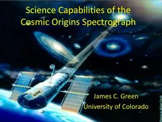
Cosmic Origins Spectrograph. St éphane Béland – ASTR-5550 – April 13, 2009. The Next UV Spectrograph for the Hubble Space Telescope. Scientific Goals. What is the large-scale structure of matter in the Universe? How did galaxies form out of the intergalactic medium?

E N D
Cosmic Origins Spectrograph StéphaneBéland – ASTR-5550 – April 13, 2009 The Next UV Spectrograph for the Hubble Space Telescope
Scientific Goals • What is the large-scale structure of matter in the Universe? • How did galaxies form out of the intergalactic medium? • What types of galactic halos and outflowing winds do star-forming galaxies produce? • How were the chemical elements for life created in massive stars and supernovae? • How do stars and planetary systems form from dust grains in molecular clouds? • What is the composition of planetary atmospheres and comets in our Solar System (and beyond)? COS will help answer some fundamental questions:
Scientific Goals • The study of the origins of large scale structure in the universe, the formation and evolution of galaxies, and the origin of stellar and planetary systems and the cold interstellar medium. • Measure the structure and composition of the ordinary matter concentrated in the ‘cosmic web’ by observing Lyα forest at low redshifts • The cosmic web is shaped by the gravity of the underlying cold dark matter, while ordinary matter serves as a luminous markers of the filaments. • Will observe faint distant quasars with absorption features from the cosmic web material (composition and its specific location in space) • Observations covering vast distances across space and back in time, will provide information on both the large-scale structure of the universe and the progressive changes in chemical composition of matter, as the universe has grown older
COS on HST • COS will replaced COSTAR (optical corrector) during next Servicing Mission 4 – May 12, 2009
COS Instrument Description • Designed for ultraviolet (115-320 nm) spectroscopy of faint point sources with a resolving power of ~1,550 to 24,000 • Optimized for high sensitivity and moderate spectral resolution of compact objects (stars, quasars, etc.). • COS has 2 channels: • Far Ultraviolet (FUV) covering 115 – 205nm with 3 gratings • Near Ultraviolet (NUV) spanning 170 – 320nm with 4 gratings, plus an imaging mode for target acquisition.
COS Instrument Description • Material reflectivity is low (~75%) in the FUV: minimize number of optics. • Slit-less spectrograph: 2.5” aperture lets ~95% of HST aberrated light to enter COS • FUV: modified Rowland Circle spectrographs with holographically ruled aspheric concave grating focuses, diffracts and corrects both the HST spherical aberration and aberrations from extreme off-Rowland layout. • Light is focused onto two 85x10 mm cross delay line micro-channel plate detectors. • FUV detector is curved to match the spectrograph’s focal plane
COS Instrument Description • NUV channel has 3 medium and 1 low resolution gratings • Imaging mode with ~1.0 arc second un-vignetted FOV • Modified Czerny-Turner design: collimated light fed to flat grating, followed by 3 camera mirrors which direct the diffracted light onto three separate regions on a 25x25 mm Multi Anode Microchannel Array (MAMA) detector. • The imaging mode is primarily intended for target acquisition (0.0236 “/pixel over ~2”)
COS Instrument Description FUV Rowland-Circle Spectrograph (curved focal plane) NUV Czerny-Turner Spectrograph
Holographic Grating • Fabrication of holographic gratings: • highly-polished and precisely-figured blanks • coated with a layer of photosensitive material • exposed to fringes created by the interference of two coherent laser beams • chemical treatment of the photosensitive layer dissolves exposed areas, forming grooves in relief. • Different design and configuration of holographic recordings provide: • plane and concave gratings (parallel grooves, uniformly spaced) • variable-spaced grooves gratings for full aberration correction • Holographic recording geometry requires very stringent optomechanical stability • The shape of the grooves produced by holographic recording is typically sinusoidal or pseudo sinusoidal (very low scatter but lower groove efficiency ~52% for COS) • Ion etching can sculpt the shape of the grooves on a holographic master grating to increase efficiency
COS Instrument Description • Wavelength calibration platform (2 PtNe + 2 Deuterium) • Focus adjustment through OSM1 • Wavelength range by rotating OSM2 or OSM2 • Aperture mechanism: • PSA, WCA, BOA (ND2), FCA • Can be moved in cross-dispersion: livetime adjustment • NCM2: mirror and rear-view mirror
OSM Drift – Tag Flash • Thermal-Vacuum tests have shown residual drift of OSM mechanisms after position reached (relaxation) • To keep track of drift, calibration lamp is turned on numerous times during exposure • Drift can be corrected for Time-Tag data only
Target Acquisition • Slit-less: absolute wavelength position on detector depends on location of target inside 2.5” aperture • Sophisticated FSW algorithms available to ensure accurate centering • ACQ/SEARCH: spiral pattern search by taking individual exposures at each point in a square grid pattern (dispersed or imaging). Returns to CENTER=FLUX-WT, or FLUX-WT-FLR, or BRIGHTEST • ACQ/PEAKXD: centers target in dispersed-light spectrum in the direction perpendicular to dispersion by moving target across aperture and returning to brightest location • ACQ/PEAKD: centers target along dispersion by taking individual exposures at each point in a closely-spaced linear pattern along dispersion. Returns to CENTER=FLUX-WT, or FLUX-WT-FLR, or BRIGHTEST • ACQ/IMAGE: NUV image of the field after the initial HST pointing, determines the telescope offset needed to center the object (some targets may be too bright for imaging) • Requires precise knowledge of WCA-PSA separation: varies with installation uncertainties – orbit verification
FUV Detector • FUV detector is a windowless XDL (cross delay line) photon-counting Micro-Channel-Plate device • Optimized for 1150 to 1775 Å, with a cesium iodide photocathode • Surface is curved (r=826 mm) to match the curved focal plane. • Photons striking the photocathode produce electrons which are amplified by MCPs. • 3 curved MCP in a stack for each segment. • Output electron cloud is several mm in diameter when it lands on the delay line anode • Each anode has separate traces for the dispersion (x) and cross-dispersion (y) axes. • Position in either axis is determined by difference in arrival times between the two ends of the delay line
FUV Detector • Time-Tag or ACCUM mode: {time, x, y, ph} or 2D image (counts at each “pixels”) • No physical pixels: location on detector determined by electronic timer (~6 x 24μm pixel) • Pixel location dependent on temperature of electronics • Injected STIM pulses used to correct for temperature drifts • Geometric distortion depends on assembly of detector • ACCUM mode for bright objects (limited by on board memory) • Gain sag with photocathode depletion: the brighter the source, the faster the gain drops • Dark counts ~1.5e-6 count/sec/pixel • Grid shadows, hot spots, dead spots, livetime correction, pulse height filtering, OSM drift
FUV Detector Geometric Distortions Pixel size variations for segment A of the FUV detector in: a) dispersion, b) cross-dispersion direction.
NUV Detector • NUV detector is a MAMA (Multi-Anode Micro-channel Array) photon-counting device • Semi-transparent cesium telluride photocathode on a magnesium fluoride window (1150-3200Å) • Photons striking the photocathode produce electrons which are amplified by MCPs. • 25.6mmx25.6mm into 1024x1024, 25μm pixels • Pixel location determined by anode array – fix pixel location • Time-Tag or ACCUM mode: {time, x, y} (no ph) or 2D image (counts at each “pixels”) • No temperature correction and geometric distortions smaller than resolution
NUV Detector • MAMA gain sag with electron extraction • Dark counts ~2.6e-6 count/sec/pixel • Each stripe only covers a non-contiguous portion of the spectra • Many central wavelengths settings to get full coverage: • G185M: 1670-2127Å in 15 settings • G225M: 2070-2527Å in 13 settings • G285M: 2480-3229Å in 17 settings • G230L: 1334-3560Å in 4 settings • Deadtime effect with high count rates
COS Observing Strategy • Identify science requirements and select the basic COS configuration to satisfy those requirements. • Estimate exposure time for required S/N and check the feasibility, including count-rate, data volume, counter rollover, and bright-object limits. • Identify any additional non-science (target acquisition, peakup, and calibration) exposures required. • Determine the total number of orbits required, taking into account all overheads.
COS Exposure Time Calculator (ETC) • Spectroscopy • Calculates count rates and S/N for a simulated spectrum of ONE source in a COS spectroscopic observation. • Spectroscopy Target Acquisition • Calculates count rates and S/N for a simulated bandpass of ONE source in a COS spectroscopic target acquisition observation. • Imaging • Calculates count rates and S/N for a simulated image of ONE source in a COS imaging observation • Imaging Target Acquisition • Calculates count rates and S/N for a simulated bandpass of ONE source in a COS imaging TA (ACQ/Image or ACQ/Search with a mirror) observation • COS Team ETC Help and Release Notes • http://etc.stsci.edu/aptServer/
COS Astronomer’s Proposal Tool (APT) • Software use to submit HST Phase I and II proposals • Integrated toolset consisting of: • Editors for filling out proposal information • Orbit Planner for determining feasibility in Phase II • Visit Planner for determining schedulability, diagnostic and reporting tools • Bright Object Protection Tool • Integrated tool based on Aladin for viewing exposure specifications overlaid on FITS images and querying the HST Archive via StarView. • Downloadable from: • http://www.stsci.edu/hst/proposing/apt