Download
1 / 38
380 likes | 380 Views
This lecture discusses the requirements and challenges in designing readout electronics for the ATLAS detector, including low noise, high speed, low power, and large dynamic range. It also explores different technologies such as diamond and compound semiconductors.

E N D
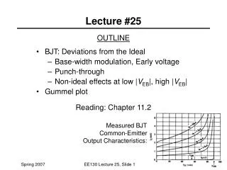
ATLAS Detector 2T solenoid, toroid system Tracking to |η|=2.5, calorimetry to |η|= 4.9
Low noise High speed Low power Large dynamic range High reliability Radiation hardness Low material Readout electronics : requirements Low cost ! (and even less)
Overview of readout electronics –Front End Most front-ends follow a similar architecture fC V V V bits Analog memory FIFO DSP… Preamp Detector Shaper ADC • Very small signals (fC) -> need amplification • Measurement of amplitude and/or time(ADCs, discr, TDCs) • Several thousands to millions of channels
Example -Liquid Argon Calorimeter Measures total energy deposited by electromagnetic showers (electrons, photons) by sampling the ionization of liquid Argon generated by electrons in the shower. Shower – sequential emission of photons and photon conversions into electron-positron pairs. Total collected charge is proportional to the deposited energy. Need to collect the charge with 0.1% precision.
Requirements of ATLAS LAr FEB • read out ~ 220k channels of calorimeter • dynamic range - 16 bits (216 = 65,536) • measure signals at bunch crossing frequency of 40 MHz(i.e., every 25 ns) • charge collection time ~ 400 ns • store signals during L1 trigger latency of ≈ 2.5 μs (100 bunch crossings) • digitize signal and read out 5 samples/channel at L1 rate of ~ 100 kHz • measure deposited energies with resolution < 0.25% • measure time of energy deposition with resolution << 25 ns • high density (128 channels per board) • low power (~ 0.8 W/channel) • high reliability over expected lifetime of > 10 years • must tolerate expected radiation levels (10 yrs LHC, no safety factors) of: • TID 5 kRad • NIEL 1.6 1012 n/cm2 (1 MeV eq.) • SEU 7.7 1011 h/cm2 (> 20 MeV)
The need for triggerData Flow from ATLAS as of 2010 40 MHz (~PB/sec) level 1 - special hardware 75 KHz (75 GB/sec) level 2 - embedded processors 5 KHz (5 GB/sec) level 3 - PCs ATLAS: 9 PB/y ~ one million PC hard drives! 100 Hz (100-400 MB/sec) data recording & offline analysis
Aside - Radiation Damage Damage due to non-ionizing energy loss (NIEL) Atomic displacement caused by massive particles (p, n, π) Damage due to ionizing energy loss – Proportional to absorbed radiation dose – 1 Gy = 1 J/kg = 100 rad = 104 erg/g (energy loss per unit mass) – Trap of ionization induced holes by “dangling bond” at Si-SiO2 interface In digital electronics a scattered Si nucleus may cross the boundary of a transistor and change its state –change from 0 to 1 or from 1 to 0. This is a transient effect SEU as the transistor operates correctly afterwards. Important for data transfer links. Solutions: triple links with voting circuit, special encoding, rad-tolerant/hard chip design Technology.
Radiation hard diamond detectors Poly-crystalline and single crystal • Competitive (to Si), used in several radiation monitor detectors • Large band gap (x5 Si) -> no leakage current, no shot noise • Smaller εr (x 0.5 Si) -> lower input capacitance and lower thermal and 1/f noise • Small Z=6 →large radiation length (x2 in g/cm2) • Narrower Landau distribution (by 10%) • Excellent thermal conductivity (x15) • Large wi (x 3.6) →smaller signal charge • poly-CVD diamond wafers can be grown >12 cm diameter, >2 mm thickness. • Wafer collection distance now typically 250μm (edge) to 310μm (center). • 16 chip diamond ATLAS modules • sc-CVD sensors of few cm2 size used as pixel detectors 16 chip diamond ATLAS modules
Common semiconductors Germanium: – Used in nuclear physics – Needs cooling due to small band gap of 0.66 eV (usually done with liquid nitrogen at 77 K) Silicon: – Can be operated at room temperature (but electronics requires cooling) – Synergies with micro electronics industry – Standard material for vertex and tracking detectors in high energy physics Diamond (CVD or single crystal): – Large band gap (requires no depletion zone) – Very radiation hard – Disadvantages: low signal and high cost
Compound Semiconductors Compound semiconductors consist of – two (binary semiconductors) or – more than two atomic elements of the periodic table. IV-IV- (e.g. SiGe, SiC), II-V- (e.g. GaAs) II-VI compounds (CdTe, ZnSe) Important III-V compounds: – GaAs: Faster and probably more radiation resistant than Si. Drawback is less experience in industry and higher costs. – GaP, GaSb, InP, InAs, InSb, InAlP " important II-VI compounds: – CdTe: High atomic numbers (48+52) hence very efficient to detect photons. – ZnS, ZnSe, ZnTe, CdS, CdSe, Cd1- xZnxTe, Cd1-xZnxSe
Overview of ATLAS LAr FEB • functionality includes: • receive input signals from calorimeter • amplify and shape them • store signals in analog form while awaiting L1 trigger • digitize signals for triggered events • transmit output data bit-serially over optical link off detector • provide analog sums to L1 trigger sum tree
DMILL AMS DSM COTS Overview of main FEB components • 10 different custom rad-tol ASICs, relatively few COTs 128 input signals 32 0T 32 Shaper 32 SCA 16 ADC 8 GainSel 1 MUX 1 fiber to ROD Analog sums to TBB 2 LSB 2 SCAC 1 Config. 1 GLink TTC, SPAC signals 20 Vregs 2 DCU 7 CLKFO 1 TTCRx 1 SPAC
Challenges General Signals are generated at cryogenic temperature (~70K) and readout at room temperature transmission lines Signals are small need pre-amplification Charge collection time is long (400 ns) in comparison with beam crossing (25 ns). Sequential decays add up additional charge (pile-up) • Need to look at the early part of the signal with fast shaping time. Signals are small (few nV) and co-exist with digital signals on the readout board need special noise control. System issues Cables take valuable space and reduce hermeticity of the detector Space on the detector is confined need low power consumption (100W/board) and water cooling Ground loops – long signal cables emit radiation Optical readout fibers, special grounding rules, stable power supplies
ATLAS LArg Front-end Optical Data Link Integrated: ~400 mm Receiving side Transmitting side
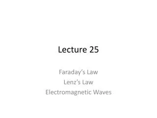
3 Data acquisition and trigger generaloverview The task of TDAQ (Trigger and Data Acquisition) system is to •Acquire data and process it •Make a decision •Store it if the decision is true
4 Read Out/Front EndElectronics •Detector signal can be in the form of charge collected in a short time duration because of the particle passing through the detector. •Main steps for readout electronics are: ▫Amplification ▫Pulse Shaping ▫Analog to Digital Conversion ▫Calibration •Most of the electronic components are specific to the type of detector.
5 Amplification •The actual signals generated in most of the detectors are very small. The amplification ▫improves the signal resolution and ▫improves signal to noise ratio •Using a simple amplifier, the input voltage depends on the detector capacitance. Detector capacitance may vary with operating point. Qs V = i Cd +Ci Qs : SignalCharge Cd : DetectorCapacitance Ci : Input Capacitance of theAmplifier
6 Charge Sensitive Amplification •Introducing a feedback capacitor in the amplifier circuit. •Output voltage gain now, depends on the feedback capacitor value.
7 Signal to Noise Ratio •Improving Signal to Noise Ratio improves the minimum detectable signal. •The need for signal to noise optimization depends on the relative fluctuation in the measurement. CaseI Signal to Noise Optimization Needed CaseII
8 Pulse Shaping ■Reduce signal bandwidth – broadening the signal in time –Fast rising signals have large bandwidth. –it is possible to cut away part of the noise after broadening. ■Reduce pulse width –Avoid overlap between successive pulses. ■The actual pulse shaping depends largely on the type of measurement.
9 Analog to Digital Conversion •Digitization – encode the analog entity into a digital representation to allow further processing and storage. •Simplest implementation is a Flash ADC. •Input Voltage is compared with M different fractions of a reference voltage. •The result is N-bit encoded binary. FlashADC
10 ADC Characteristics •least Significant Bit (LSB) : Minimum Readable input voltage (Vmax/2N) •Quantization Error : Finite size of the voltage unit. ±LSB/2 •Dynamic Range : Possible Range of Operation, Vmax/LSB (expressed in bits). •Many different techniques of ADCs exist, because of trade off between speed, resolution, power consumption and cost.
11 Time Measurement : TDC Single Hit TDC: If a noise pulse hits before the signal - the measurement islost
12 Multi hitTDC •Counter is on for the time period defined by gate. •Each hit forces the current value of the counter to be stored in a memory. •Additional logic is needed to separate out the different readings. •Real TDCs provide advanced functionalities for fine-tuning the hit-trigger matching.
13 Calibration • •Experimental measurement is usually related to the actual physics quantity of interest. • •Calibration : Finding the relation parameters which transform the measured quantity into the physics quantity of interest. • •Calibration factors usually depend on the detector layout and can also change with ageing/beam conditions. • •Energy in a channel of ATLAS tile calorimeter is given by Integrator Readout (Cs & Particles) Calorimeter Tiles Photomultiplier Tubes Particles Digital Readout (Laser & Particles) Charge injection(CIS) Laserlight 137Cs source
14 •A represents the measured energy in ADC counts. •CADC->pC is the conversion factor of ADC count to charge and is determined by charge injection system. •CpC->GeV is the conversion factor of charge to energy and is determined by EM scale studies. •CCs corects for residual non-uniformities in the detector channels done using 137Cs source scans. •Claser corrects for non-linearities of the PMT response measured by Laser Calibration System.
16 Basic DAQ: Physics Trigger •While measuring a stochastic physics process, a Trigger is a system which rapidly decides if the observed event is interesting and initiates the data acquisition process. •Delay compensates for the trigger latency ie. Time needed to reach a decision. Since the process to be measured, is stochastic, an interesting event can occur during the processing time of the DAQ.
18 DAQ Deadtime and Efficiency •DAQ deadtime is the system requires to process an event, without being able to handle other triggers. ν – average DAQ frequency, τ – time needed for processing an event f – average frequency of interesting events •Due to fluctuations in the stochastic event, DAQ efficiency is always less than 100% •In order to obtain ν≈f, fτ<<1 --> τ<<1/f •In order to cope with the input fluctuation, we have to overdesign the DAQ.
20 Basic DAQ forColliders •Particle Collisions happen at regular intervals. •Trigger rejects uninteresting events based on physics criteria. •Triggers for good events are eventually unpredictable and hence de-randomization is needed.
21 Large DAQ:constituents
LAr Barrel FE-BE integration LAr ROD system in USA15 LAr FE crate on cryostat
ATLAS event simulation and reconstruction 40 MHz - frequency of bunch crossing ~20 pp collisions per bunch crossing ~1000 tracks in detector per bunch crossing
Tier2 Center Tier2 Center Tier2 Center Tier2 Center Tier2 Center HPSS HPSS HPSS HPSS Data Grids for High Energy Physics CERN/Outside Resource Ratio ~1:2Tier0/(~ Tier1)/(~ Tier2) ~1:1:1 ~PByte/sec ~100-400 MBytes/sec Online System Offline Farm,CERN Computer Ctr ~25 TIPS Tier0 +1 10+ Gbits/sec HPSS Tier 1 France Italy UK BNL Center Tier 2 ~2.5+ Gbps Tier 3 Physicists work on analysis “channels” Each institute has ~10 physicists working on one or more channels Institute ~0.25TIPS Institute Institute Institute 100 - 10000 Mbits/sec Physics data cache Tier 4 Workstations ATLAS version from Harvey Newman’s original
Tier2 Center Tier2 Center Tier2 Center Tier2 Center Tier2 Center HPSS HPSS HPSS HPSS Data Grids for High Energy Physics CERN/Outside Resource Ratio ~1:2Tier0/( Tier1)/( Tier2) ~1:1:1 ~PByte/sec ~100-400 MBytes/sec Online System Offline Farm,CERN Computer Ctr ~25 TIPS Tier0 +1 10+ Gbits/sec HPSS Tier 1 France Italy UK BNL Center Tier 2 ~2.5+ Gbps Tier 3 Physicists work on analysis “channels” Each institute has ~10 physicists working on one or more channels Institute ~0.25TIPS Institute Institute Institute 100 - 10000 Mbits/sec Physics data cache Tier 4 Workstations ATLAS version from Harvey Newman’s original
Data Flow from ATLAS 40 MHz (~PB/sec) level 1 - special hardware 75 KHz (75 GB/sec) level 2 - embedded processors 5 KHz (5 GB/sec) level 3 - PCs ATLAS: 9 PB/y ~ one million PC hard drives! 100 Hz (100-400 MB/sec) data recording & offline analysis
ATLAS Parameters • Running conditions in the early years: >3 years delay • Raw event size ~2 MB • 2.7x10⁹ event sample 5.4 PB/year, before data processing • Reconstructed events, Monte Carlo data • ~9 PB/year (2PB disk); CPU: ~2M SI95 (today’s PC ~ 20 SI95) • CERN alone will provide only 1/3 of these resources…how will we handle this?
ESD ESD ESD ESD ESD Physics Analysis Event Tags Tier 0,1 Collaboration wide Event Selection Analysis Objects Calibration Data Analysis Processing Raw Data Tier 2 Analysis Groups PhysicsObjects StatObjects PhysicsObjects StatObjects PhysicsObjects StatObjects Tier 3, 4 Physicists Physics Analysis