Download
1 / 51
510 likes | 598 Views
Numerical method on NICAM Hirofumi Tomita Research Institute for Global Change JAMSTEC. Contents. Numerical method on NICAM Dynamical core Horizontal discretization Icosahedral grid Modified by spring dynamics( Tomita et al. 2001, 2002 JCP) Nonhydrostatic framework

E N D
Numerical method on NICAM Hirofumi Tomita Research Institute for Global ChangeJAMSTEC
Contents • Numerical method on NICAM Dynamical core • Horizontal discretization • Icosahedral grid • Modified by spring dynamics( Tomita et al. 2001, 2002 JCP) • Nonhydrostatic framework • Mass and total energy conservation • ( Satoh 2002, 2003 MWR ) • Computational strategy • Domain decomposition in parallel computer • Example of computational performance • ES ( vector-based machine ) • T2K TSUKUBA ( scalar-based machine ) • Stretched-NICAM • Use of NICAM as the regional model • Summary
NICAM • Nonhydrostatic ICosahedral Atmospheric Model • Why Nonhydrostatic? • General problem for current AGCMs • Cumulus parameterization • One of ambiguous factors • Need to increase resolution up to cloud size( ~1km ) • Hydrostatic assumption : invalid • Why ICosahedral? • Spectral method : not efficient in high resolution simulations. • Legendre transformation • Massive data transfer between computer nodes • Latitude-longitude grid : the pole problem. • Severe limitation of time interval by the CFL condition. • The icosahedral grid:homogeneous grid over the sphere • To avoid the pole problem. • Why Atmospheric Model?
Grid generation Start from the spherical icosahedron. (glevel-0) Connection of the mid-points of the geodesic arc 4 sub-triangle (glevel-1) Iteration of this process A finer grid structure (glevel-n)STD-grid # of gridpoints 3.5km grid: 11 interations are required. Grid Generation Method (0) grid division level 0 (1) grid division level 1 (2) grid division level 2 (3) grid division level 3
Grid arrangement • Arakawa A-grid type • Velocity, mass • triangular vertices • Control volume • Connection of center of triangles • Hexagon • Pentagon at the icosahedral vertices • Advantage • Easy to implement • Less computational mode • Same number of grid points for vel. and mass • Disadvantage • Non-physical 2-grid scale structure • E.g. bad geostrophic adjustment Glevel-3 grid & control volume
Horizontal differential operator • e.g. Divergence • Vector : given at Pi • Interpolation of u at Qi • Gauss theorem 2nd order accuracy? NO Allocation points is not gravitational center ( default grid )
Error distribution of div U Error of divergence operator Area of CV • Error of div operator • Large error on the original icosahedral arc • Fractal distribution • Generation of grid noise • Distribution of CV area • Fractral distribution GUESS: smoothness of CV Reduction of grid noise
Modified Icosahedral Grid (1) • Reconstruction of grid by spring dynamics • To reduce the grid-noise • STD-grid :Generated by the recursive grid division. • SPRING DYNAMICS :Connection of gridpoints by springs
Modified Icosahedral Grid (1) • SPR-grid • Solve the spring dynamics The system calms down to the static balance • Construction of CV • Connection of the center of triangles • One non-dimensional parameter b • Natural length of spring • Should be tuned!
Dependency of b on homogeneity The ratio of lmax/ lmin against the parameter b The standard grid lmax/lmin 1.34. • The spring grid • lmax/lmin depends on b and glevel. • If b =1.2, lmax/lmin1.24.
Modified Icosahedral Grid (2) • Gravitational-Centered Relocation • To make the accuracy of numerical operators higher • SPR-grid:Generated by the spring dynamics. ● • CV:Defined by connecting the GC of triangle elements. ▲ • SPR-GC-grid:The grid points are moved to the GC of CV. ● The 2nd order accuracy of numerical operator is perfectly guaranteed at all of grid points.
Improvement of error distribution - Area of CV- Error of divergence • STD-grid • Area of CV • Fractral distributiondue to recursive division • Error of divergence • Fractral distribution error • Generation of grid noise • SPR-GC-grid • Area of CV • Smooth distribution • Error of divergence • Smooth distribution Reduction of grid noise STD-grid SPR-GC-grid
Improvement of accuracy of operator • Test function • Heikes & Randall(1995) • Error norm • Global error • Local error
Test Case for SWM • Shallow water equations • Vector invariant form • A Standard Test Case • Williamson et al. (1992, JCP) • TEST CASE2 • Solid body rotation test • TEST CASE5 • Unsteady, nonlinear but deterministic test with mountain
TEST CASE 2 (1) • Test configuration • Initial condition • Solid body rotation • Geostrophic balance • Purpose • How does the model maintain the initial state? • Integration time • 5 days • Monitor • Time evolution of L_inf normof surface height
TEST CASE 2(2) Time evolutionl∞norm • STD-grid(---) • No modification of grid • Large error from the initial stage • STD-GC-grid(---) • Only GCR modification • Small error just in 1 day • Large error from 2 day • Grid-noise • SPR-GC-grid(---) • Spring dyn & GCR • Small error during 5 days No grid-noise • Numerical condition • Resolution :glevel-5 • Integration:5day • numerical diffusion: none
TEST CASE 5 (0) t=0 day (1) t=5 day (2) t=10 day (3) t=15 day Result : glevel5 SPR-GC grid without viscosity • Test Configuration • Initial condition • Solid body rotation • Mountain at the mid-latitude • Integration • 15 days • Purpose • Check the conservationTotal energyPotential enstrophy No grid noise
TEST CASE 5 (2) • Grid refinement result ( SPR-GC grid ) • Resolution:glevel-4,5,6,7 • Numrical diffusion : NONE Conservation of total energy Conservation of potential enstrohpy Error : reduction by a factor of 4 in the 2nd order
Design of our non-hydrostatic modeling • Governing equation • Full compressible system • Acoustic wave Planetary wave • Flux form • Finite Volume Method • Conservation of mass and energy • Deep atmosphere • Including all metrics terms and Coriolis terms • Solver • Split explicit method • Slow mode : Large time step • Fast mode : small time step • HEVI ( Horizontal Explicit & Vertical Implicit ) • 1D-Helmholtz equation
Governing Equations L.H.S. : FAST MODE R.H.S. : SLOW MODE (1) (2) (3) (4) • Metrics • Prognostic variables • density • horizontal momentum • vertical momentum • internal energy
Temporal Scheme (RK2) • Assumption : the variable at t=A is known. • Obtain the slow mode tendency S(A). • 1st step : Integration of the prog. var. by using S(A) from A to B. • Obtain the tentative values at t=B. • Obtain the slow mode tendency S(B) at t=B. • 2nd step : Returning to A, Integration of the prg.var. from A to C by using S(B). Obtain the variables at t=C HEVI solver
Small Step Integration In small step integration, there are 3 steps: • Horizontal Explicit Step • Update of horizontal momentum • Vertical Implicit Step • Updates of vertical momentum and density. • Energy Correction Step • Update of energy • Horizontal Explicit Step • Horizontal momentum is updated explicitly by HEVI Fast mode Slow mode : given
Small Step Integration (2) • Vertical Implicit Step • The equations of R,W, and E can be written as: • Coupling Eqs.(6), (7), and (8), we can obtain the 1D-Helmholtz equation for W: • Eq.(9) W • Eq.(6) R • Eq.(8) E (6) (7) (8) (9)
Small Step Integration (3) • Energy Correction Step (Total eng.)=(Internal eng.)+(Kinetic eng.)+(Potential eng.) • We consider the equation of total energy where • Additionally, Eq.(10) is solved as • Written by a flux form. • The kinetic energy and potential energy: known by previous step. • Recalculate the internal energy: (10)
Large Step Integration • Large step tendecy has 2 main parts: • Coliolis term • Formulated straightforward. • Advection term • We should take some care to this term because of curvature of the earth • Advection of momentum • The advection term of Vh andW is calculated as follows. • Construct the 3-dimensional momentum V using Vh andW. • Express this vector as 3 components as (V1,V2,V3) in a fixed coordinate. • These components are scalars. • Obtain a vector which contains 3 divergences as its components. • Split again to a horizontal vector and a vertial components.
Computational strategy(1) (0) region division level 0 (1) region division level 1 • Domain decomposition • By connecting two neighboring icosahedral triangles, 10 rectangles are constructed. (rlevel-0) • For each of rectangles, 4 sub-rectangles are generated by connecting the diagonal mid-points. (rlevel-1) • The process is repeated. • (rlevel-n) (2) region division level 2 (3) region division level 3
Computational strategy(2) • Example ( rlevel-1 ) • # of region : 40 • # of process : 10 • Situation: • Polar region:Less computation • Equatorial region:much computation • Each process • manage same color regions • Cover from the polar region and equatorial region. Load balancing Avoid the load imbalance
Computational strategy(3) Vectorization • Structure in one region • Icosahedral grid Unstructured grid? • Treatment as structured grid Fortran 2D array vectorized efficiently! • 2D array 1D array • Higher vector operation length
Computational Performance (1) • Computational performance • Depend on the many things • Computer architecture, degree of code tuning….. • Performance on the old Earth Simulator • Earth Simulator • Massively parallel super-computer based on NEC SX-6 architecture. • 640 computational nodes. • 8 vector-processors in each of nodes. • Peak performance of 1CPU : 8GFLOPS • Total peak performance: 8X8X640 = 40TFLOPS • Target simulations for the measurement • 1 day simulation of Held & Suarez dynamical core experiment
Computational Performance (2) • Scalability of our model (NICAM) • Configuration • Horizontal resolution : glevel-8 • Vertical layers : 100 • Fixed • The used computer nodes increases from 10 to 80. • Results • Green : ideal speed-up line • Red : actual speed-up line good scalability!
Computational Performance (3) • Performance against the horizontal resolution The elapse time should increase by a factor of 2. • Configuration • As the glevel increases, • # of gridpoints : X 4 • # of CPUs : X 4 • Time intv. : 1/2 Results Actually, the elapse time increases by a factor of 2.
Computer performance(4) • How about scalar-based machine • Machine : T2K tsukuba • 4 core – 4 socket Opteron cluster • Measurement • Glevel 7 : fixed • Rlevel : 1~4 changed • How does the scalability change? • How about the sustainable performance?
Scalability : comparison with ES T2K-Tsukuba: inefficient from 640 to 2560 core communication overhead? ES: ineffcient at 640 vector length is shortened.
Communication/calculation ratio One reason of degrading efficiency : communication The ration of communication against calculation: increasing from 640(rlevel3) to 2560(rlevel4)
Computational performance in a scalar machine • Another reason for degrade of efficiency at increasing rlevel • ratio of halo region against managing points ● : managing points in a region ● : halo points The caluculation: both at ● and ● • If rlevel increases, • ● : 1/4 • ● : ½ • Total caluclation does not reduce by a factor of 4. • more calculation
What combination of glevel & rlevel is the best? • Depend on the architechtue? • In T2K, it’s ok that the effective glevel ( glevel-rlevel ) is 4. • However, effective glevel 3 is not bad.
Schematic explanation • Use of NICAM as a regional model • Stretched icosahedral grid • Method to make a stretched grid • Gather the grid points in the north pole regionby an appropriate transformation function • e.g. figure 1 • Rotate the grid system to the interested region • e.g. figure 2 Figure 1 Figure2
Preferable transformation The transform function : latitude • Preferable aspect • Homogeneity in the target region • First derivative of transformation function • Constant • Isotropy in the target region • The shape of grid element • Regular triangle Regular triangle • Smoothness of the function • Avoid the reflectivity of waves • Less parameters • Many parameters • inconveinent
Isotropic transformation (1) • Transformation of latitude • Number of grid at A: N • Latitudinal circle : 2pcosf • Mean grid interval :Dq in the homogeneous grid :Df = Dq • By the transformation, latitude A latitude B • Latitudinal circle : 2pcos(f(f)) • Mean grid interval :Dq’ Require: The grid interval in the latitudinal direction is same as that of the longitudinal direction
Isotropic transformation (2) • Solution of ODE • Parameter : b (stretched factor) Same formulation as the Schmidt transformation (Schmidt,1977) Homogeneous in the target region
Example of stretched grid • Stretched grid • After the transformation • Grid interval : • 120km 12km • Default grid : glevel-6 • 120km grid intv. • Homogenious Reduction of earth radius : 1/10 1.2km grid interval
Summary • NICAM • Nonhydrostatic AGCM • For nonhydrostatic scheme, we consider the conservation of total mass and total energy. • Time spliting method • Slow mode : RK2, RK3, RK4 • Fast mode : Horizontal explicit & vertical implicit • To avoid the pole problem, we employ the icosahedral grid, which is modfied by spring dynamics. • More robust against the numerical instability. • Computational strategy • 2d-domain decomposition • ES, T2K • Stretched NICAM • We can use NICAM as the regional model without nesting technique.
Simple transformation(2) • a=1/3.2 • Generated smoothly • anisotopy over the equator • Flat triagles From the north pole From the equator From the south pole
Isotropic transformation (3) From the north pole From the equator From the south pole Schmidt transformation Simple transformation
Simple transformation(1) • Power type In the case of a=1 , identical transformation